How To Automatically Alphabetize in Google Sheets

Google Sheets and Microsoft Excel share many similar features. Those that are more familiar with Excel will find out that though most features are the same, locating them in Google Sheets can become an obstacle while familiarizing yourself with the program.

The ability to sort and filter your data, alphabetically or numerically, is one of the more commonly used features in Microsoft Excel. The same can be said for Google Sheets. However, the way to go about performing the task can be a bit different.

“I’m more familiar with Excel but my boss wants us using Google Sheets now. Organizing spreadsheets are part of the job. Can you help?”

The great part about Sheets, just like Excel, you will not have to worry about manual edits when you wish to sort or filter your data. There is a way to have them auto-sorted by column using the functions provided in the tabs or through a formula you can place directly into a cell.

Automatically Organizing Google Sheets Alphabetically

The steps below will detail how you can organize your Google Sheet data automatically. I’ll be focusing on how to do so alphabetically but the same information can also be used if you’d rather organize the data numerically.

However, before we proceed with the end goal, I’d like to get a bit more familiar with what the difference between sorting and filtering are, how to use either option for any situation that you may need them for, as well as go over filter views.

If you’ve already got a decent understanding of sorting and filtering and would just like to get to the auto-alphabetizing, you can skip further down the article. For everyone else who’d like to learn something, we’ve got a lot to cover, so let’s get started.

Data Sorting & Using Filters

As you analyze and work within Google Sheets, more and more content will begin to accumulate. This is when the ability to organize the information becomes that much more important. Google Sheets allows you to reorganize that information by sorting and applying filters to it. You can do this both alphabetically and numerically, the choice is up to you. You can also apply a filter in order to narrow down the data and even hide select portions from view.

Data Sorting

To sort the data:

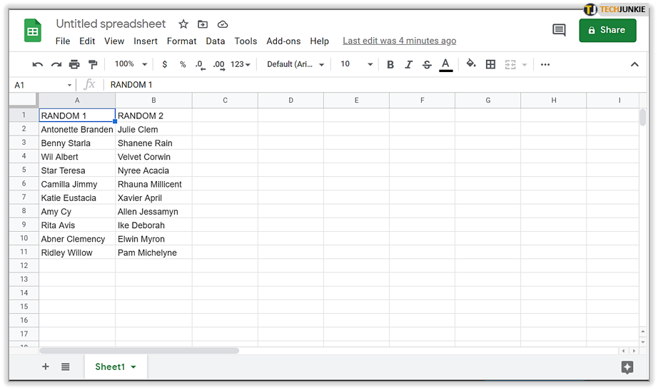
1. From your browser (Google Chrome preferred), open a spreadsheet in Google Sheets.
   
2. Highlight the cell or cells you’d like to sort.
   • You can left-click a single cell to highlight it. For multiple cells, left-click the beginning cell. Hold down Shift and then left-click in the ending cell.
   • Multiple cells can also be selected by left-clicking a cell and the holding down Ctrl and left-clicking another cell. This helps if the cells you want to be sorted are not sequential.
   • To select the entire sheet, click the top left corner of the sheet or press Ctrl+A simultaneously.
     
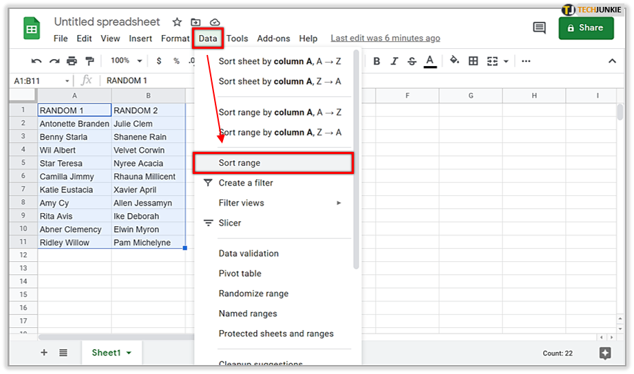
3. Next, click the “Data” tab and select Sort Range… from the options.
   
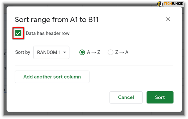
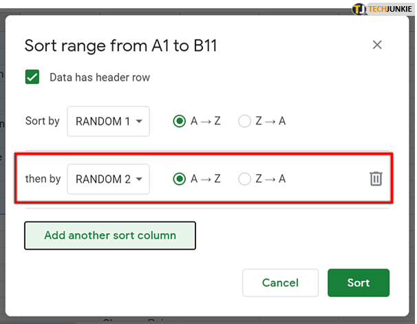
4. In the pop-up window, if your columns have titles, put a check mark in the box next to Data has header row.
   
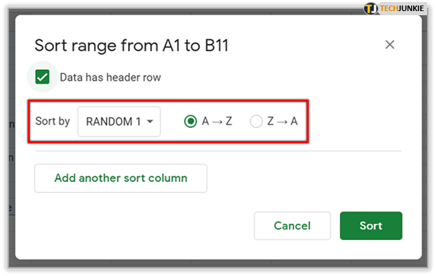
5. Select the column you first want to sort by changing the “Sort by” to that column. Then select the sorting order by clicking either the A-Z radial for descending or Z-A for ascending.
   
   • If you have an additional sorting rule you’d like to apply, click Add another sort column. The order of your rules will determine how the sorting is done.
   • You can click on the Trash icon to the right of a rule in order to delete it.
     
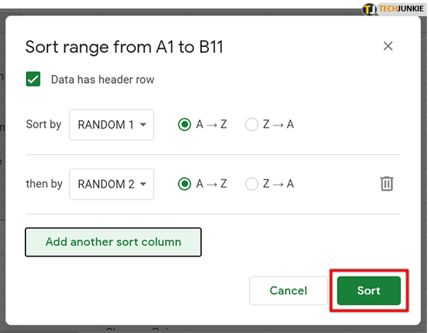
6. Finalize by clicking the Sort button and your range will be sorted according to your rules.
   

Data Filtering

Adding filters to your data will enable you to hide the data that you don’t want visible. You’ll still be able to see all of your data once the filter has been turned off. Filters and filter views both help to analyze data sets within spreadsheets.

Filters are preferred when:

• Having everyone who accesses your spreadsheet view a specific filter when opened.
• You’d like the visible data to remain sorted after a filter has been applied.

Whereas Filter Views are more useful if:

• You want to name and save multiple views.
• Multiple views are needed for others using the spreadsheet. Filters are turned on by the individual so this allows them to view different filters at the same time someone else may also be using the spreadsheet.
• Sharing different filters with people is important. Different filter view links can be sent to different people providing everyone working on the spreadsheet with the most relevant information specific to the individual.

Just remember that filters can be imported and exported as needed while filter views cannot.

Using Filters Inside A Google Spreadsheet

When a filter has been added to a spreadsheet, anyone else viewing that spreadsheet can see the filters too. This also means that anyone with edit permissions can alter the filter. A filter is a great way to temporarily hide data in a spreadsheet.

To filter your data:

1. From your browser (Google Chrome preferred), open a spreadsheet in Google Sheets.
   
2. Select the cell range you’d like to filter using the same methods as detailed in the Data Sorting section of the article.
   
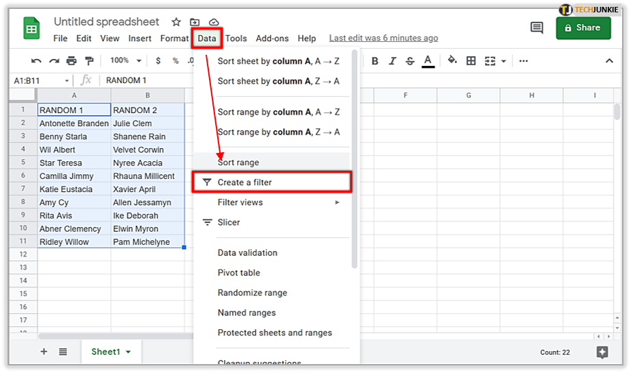
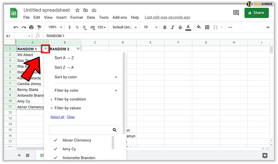
3. Click the “Data” tab and then select Create a filter. This will place a Filter icon within the first cell of the range you selected. All cells within the filter range will be encased in a green border.
   
4. Click the Filter icon to have the following filter options displayed:
   
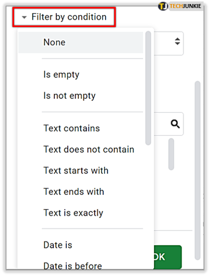
   • Filter by condition – Choose from a list of conditions or write your own. For example, if the cell is empty, if data is less than a certain number, or if the text contains a certain letter or phrase.
     
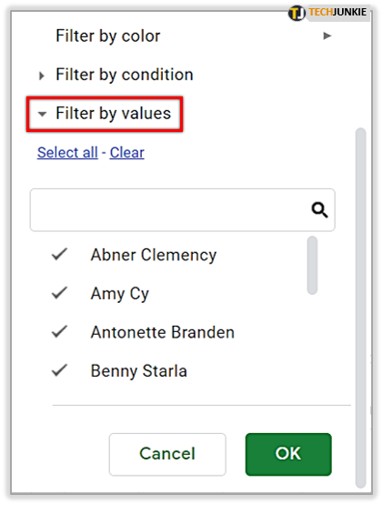
   • Filter by values – Uncheck any data points that you want to hide and click OK. If you want to choose all of the data points, click Select all. You can also uncheck all data points, by clicking Clear.
     
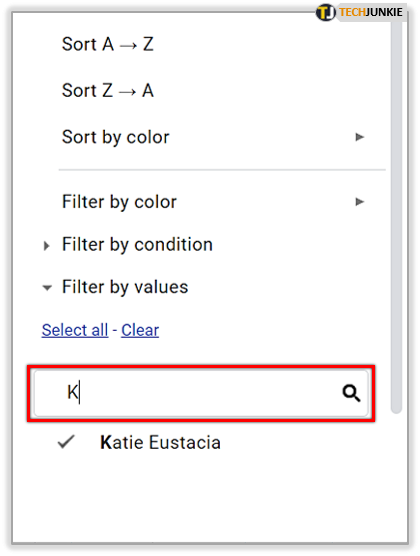
   • Search – Search for data points by typing in the search box. For example, typing “K” will shorten your list to just the names that start with K.
     
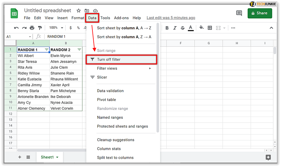
5. To disable the filter, just click the “Data” tab again and then select Turn off filter.
   • Data can be sorted while a filter is in place and enabled.
   • Only the data in the filtered range will be sorted when choosing to sort.
     

Creating A Filter View

To create, save, or delete a filter view:

1. From your browser (Google Chrome preferred), open a spreadsheet in Google Sheets.
   
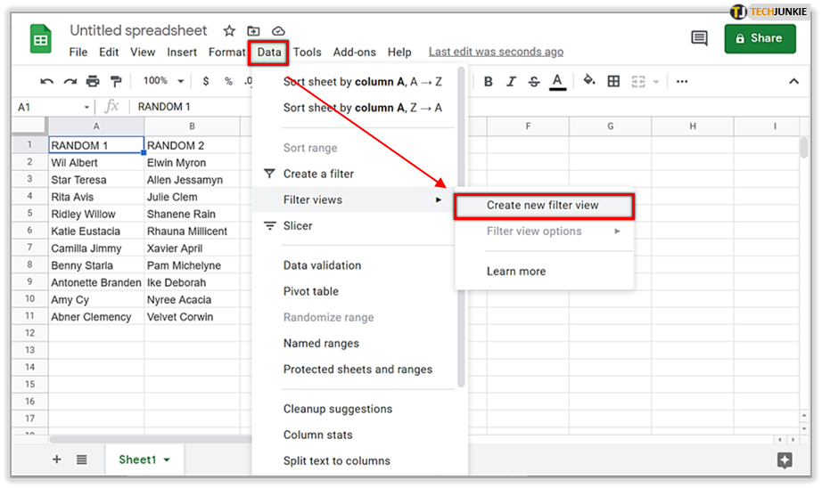
2. Click the “Data” tab and then select Filter views… followed by Create new filter view.
   
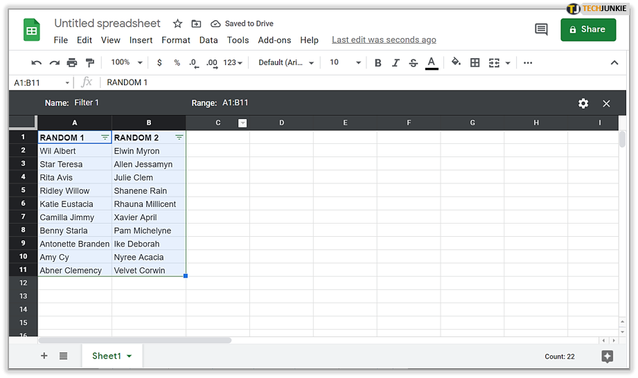
3. The filter view is saved automatically. You can now sort and filter any of the data that you wish.
   
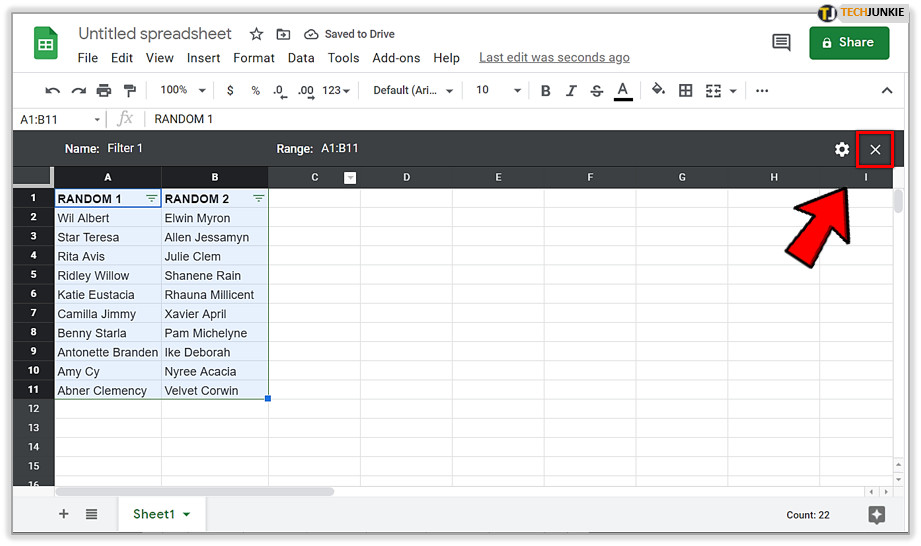
4. Close your filter view by clicking the ‘X’ in the top-right corner of the spreadsheet.
   
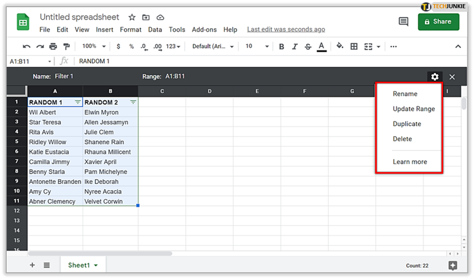
5. Click the Cogwheel icon at the top-right of the spreadsheet for one of the following options:
   
   • Rename – change the title of the filter view.
   • Update Range – This isn’t as important as you can do so directly on the filter view itself. It allows you to change the range of cells chosen for the filter view.
   • Duplicate – Creates an identical copy to the current filter view.
   • Delete – Delete the filter view.

Google Sheets: Sorting Alphabetically On Desktop

To sort a cell range alphabetically on your desktop:

1. From your browser (Google Chrome preferred), open a spreadsheet in Google Sheets.
   
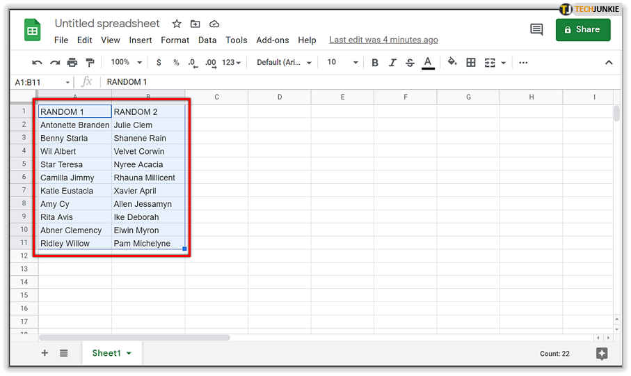
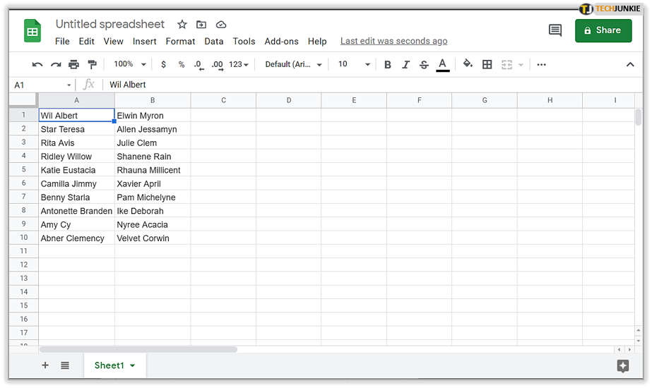
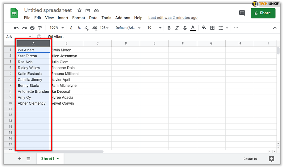
2. Select the data you want to sort one column at a time. This is important so as not to rearrange other parts of your spreadsheet that may not correlate to the range desired.
   • Highlight the top cell in your data’s column all the way down to the final cell.
     
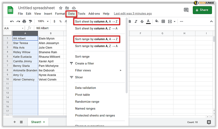
3. Click the “Data” tab and then select one of the following options:
   
   • Sort range by column [Letter], A → Z – This will sort all selected data within the range into alphabetical order without disrupting the other areas of the spreadsheet.
   • Sort sheet by column [Letter], A → Z – This adjusts all data in the spreadsheet alphabetically in correlation to the data range highlighted.
4. Either choice should now have your data rearranged into alphabetical order.
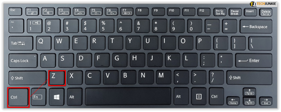
   • If you feel you’ve made a mistake, you can easily correct it by pressing Ctrl+Z (Windows) or ⌘ Command+Z (Mac) to undo the most recent data sorting.
     

Alphabetically Sort Your Data Automatically Using A Formula

Though the previous steps can be considered automatic, there is still a slight bit of manual input involved. This is perfectly acceptable for most spreadsheet users who don’t want to get too technical with formulas and functions.

However, there are some who would prefer a more “full-auto” approach to the data alphabetizing situation. You may prefer to have the data sorted automatically in a column. This means that whenever new information is put into the column, the data will automatically be updated alphabetically without disrupting the rest of the spreadsheet.

To automatically sort the column data alphabetically:

1. From your browser (Google Chrome preferred), open a spreadsheet in Google Sheets.
   
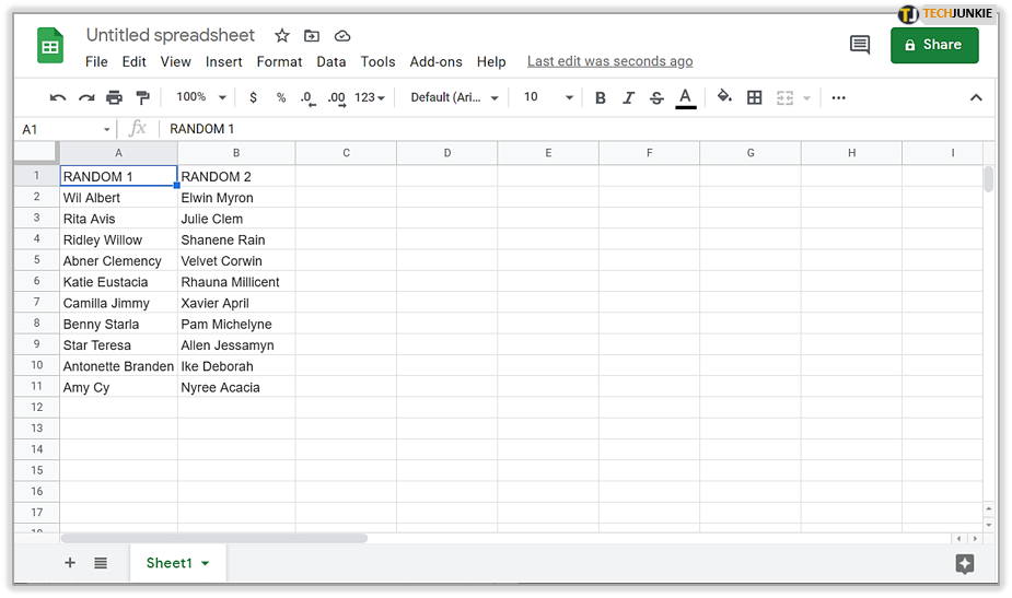
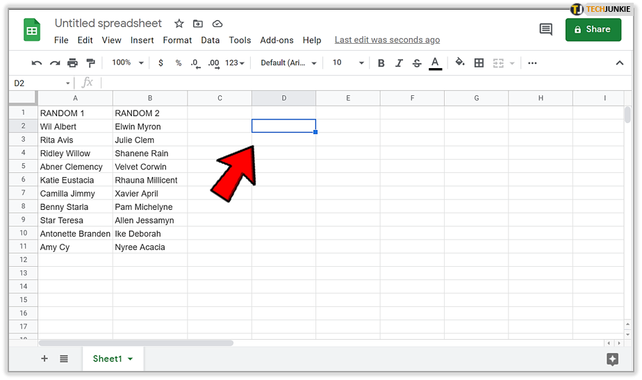
2. Highlight the cell that will display the results for the data you want automatically alphabetized.
   
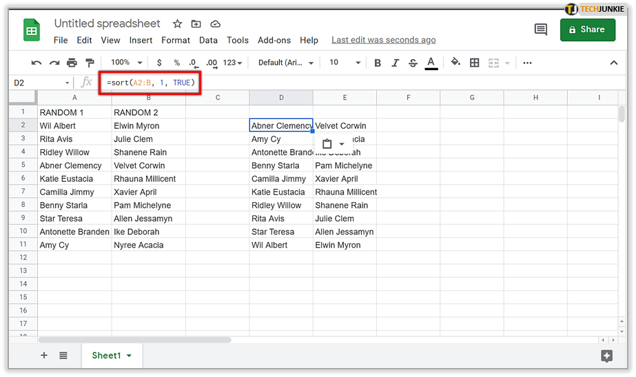
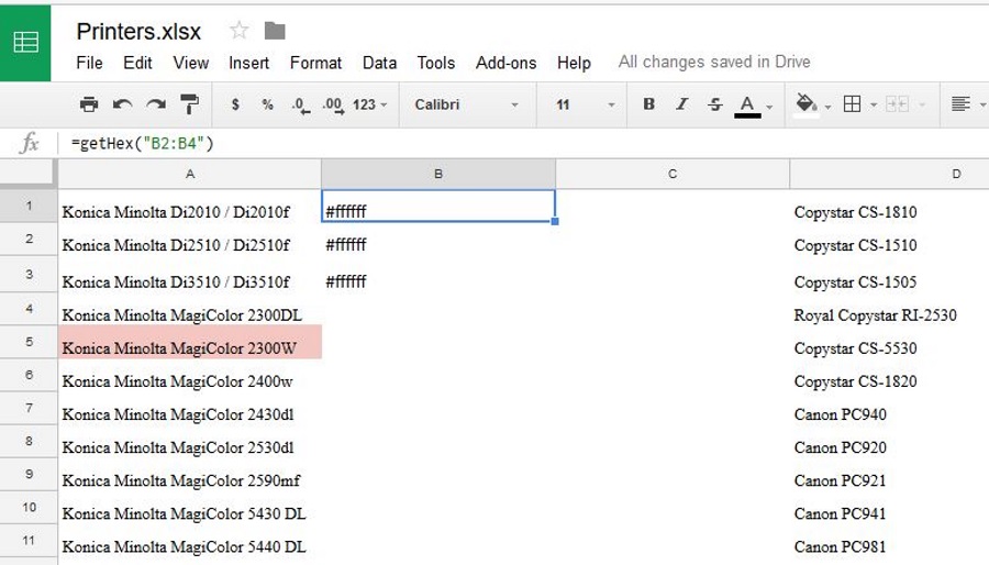
3. Inside the cell, enter in the following formula =sort(A2:B, 1, TRUE) and then press Enter.
   
   • A2:B is the desired data range that needs to be sorted. Adjust it according to your own spreadsheet needs.
   • The 1 refers to the column number that the sorted data will be based on. Again, adjust it according to the needs of the spreadsheet.
   • Data in the formula is automatically sorted in ascending order. To sort the data in descending order, change the TRUE to FALSE.

Any new or edited data entered into the column will now be sorted automatically.

Google Sheets: Sorting Alphabetically On Mobile Device

To sort a cell range alphabetically on your mobile device:

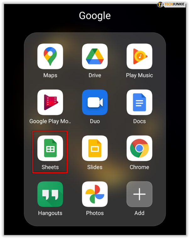
1. Launch the Google Sheets app(Android / iOS) and log in using your credentials.
   
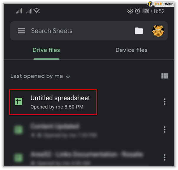
2. Select a Google Sheet to edit by tapping on the spreadsheet. You may need to scroll to find it if you have multiple Sheets saved.
   
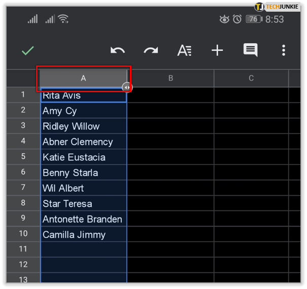
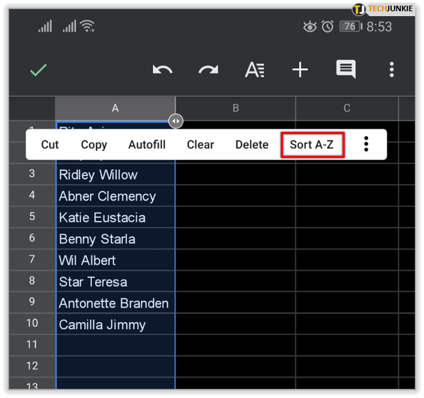
3. Locate the column with the data that you want to alphabetize and tap that column’s letter. It can be found at the top of the column. This will highlight all of the column’s data.
   
4. Tap the letter once more to pull up a small menu.
   
5. In the menu, tap on Sort A – Z option.
   
   • If using an Android mobile device, you’ll need to tap the icon that looks like three vertically (or horizontally depending on the version) stacked dots. Scroll down until you find the Sort A – Z option.

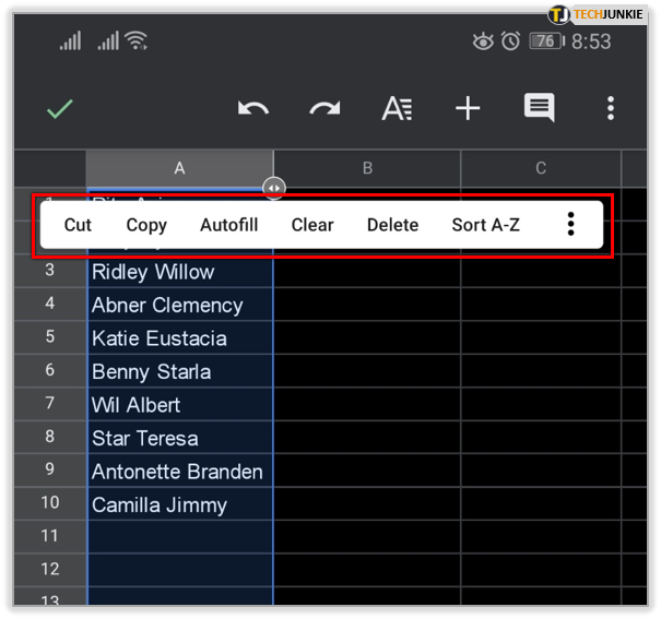
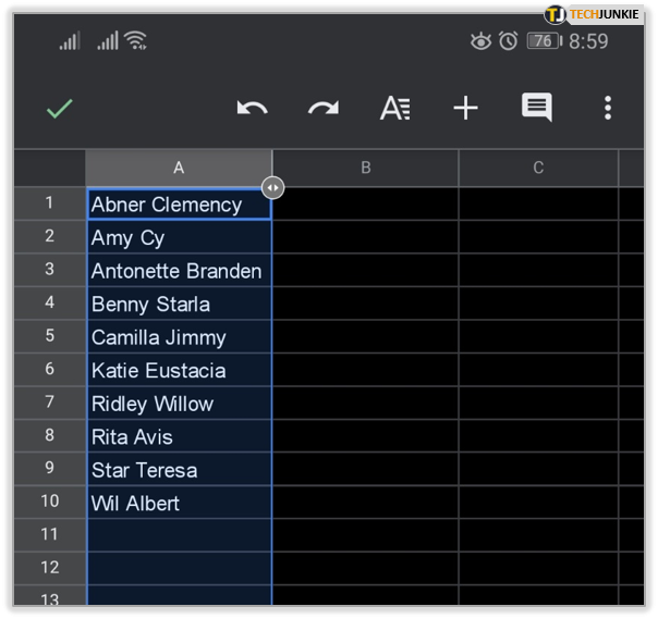
When you tap on Sort A – Z, the data within the column will be rearranged alphabetically.