

How to Automatically Group Rows in Excel

When you’re analyzing a huge amount of data, it’s always convenient to use programs like Excel to help you out. By putting your data into an Excel worksheet, you can organize and process all that information as you see fit.
Sometimes, you may just have too much data. And that can get really distracting. The best way to deal with the data you’re not currently using is to hide it. This can help you focus on the important figures that are relevant to your analysis.
In Excel, this option is called Grouping. It can be done both automatically and manually, depending on the structure of your data.
Please note that grouping is different from the “Hide” option. When you hide rows or columns and you want to print the sheet you’re working on, hidden items will not appear on the printout. Or, you may have locked your sheet for editing but forgot to unhide some rows. If you share that Excel file with someone, they won’t be able to see the hidden rows. In both of these cases, the grouped data would still be visible.
Automatic Grouping
To get the best result when automatically grouping the data, it’s good to stick to these guidelines for your dataset:
- Add column headings to the top row.
- Avoid having blank rows or columns that contain no data.
- Include summary rows for each of the subsets.
To group your data automatically, follow these steps:
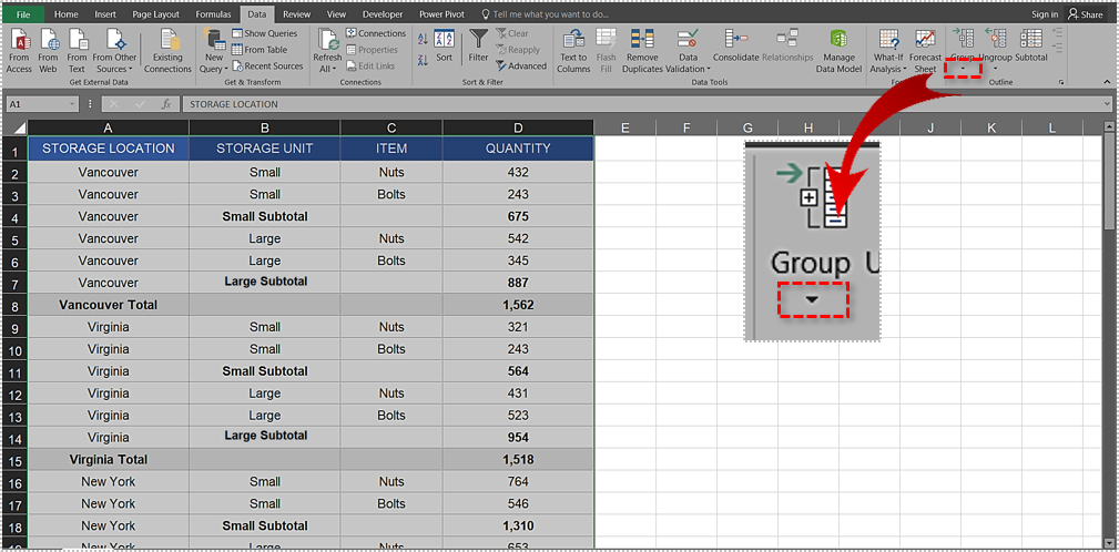
- Select any of the cells that contain data in your dataset.

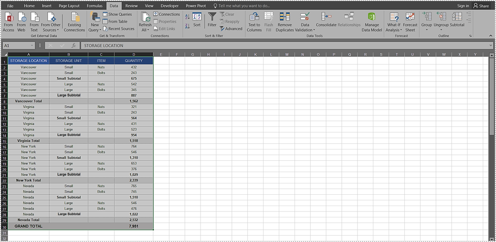
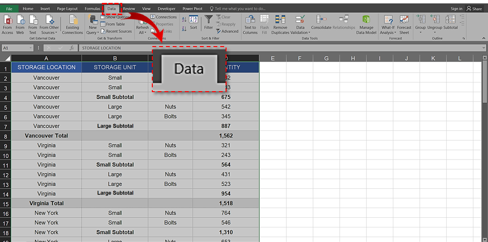
- Select the “Data” tab in the Excel menu.

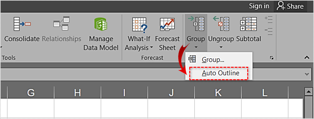
- In the “Outline” section, click on a small arrow beneath the “Group” icon.

- Select “Auto Outline”.

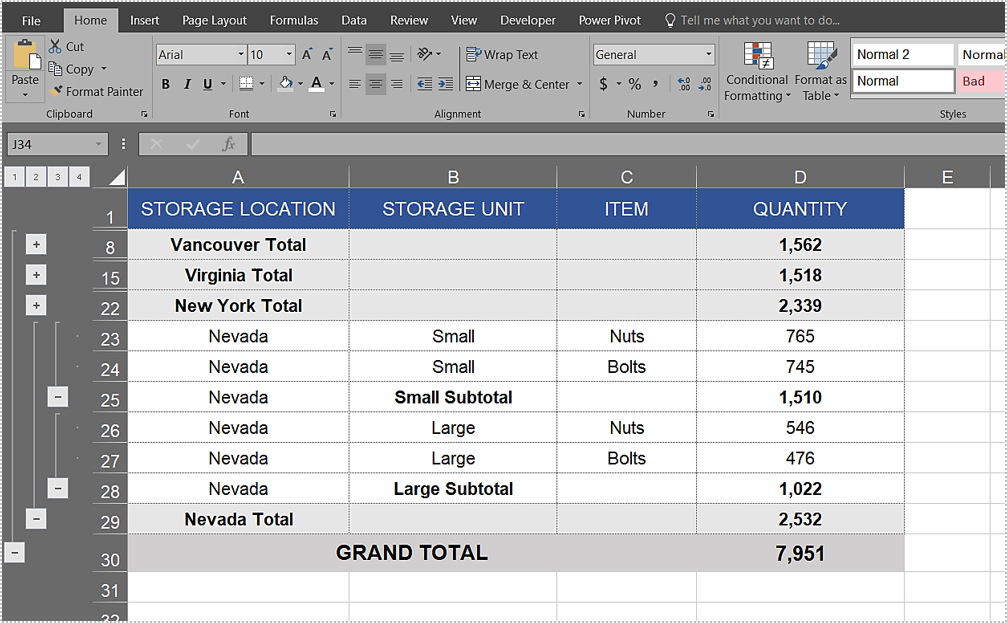
Excel will group your data and add grouping levels to the left of column A. This addition allows you to easily organize your data, by choosing which data you’d like to see and which should remain hidden for now.
If you have placed the summary rows above the rows that contain grouped units, you’ll have to adjust your grouping options. This is done after you have performed the above steps.
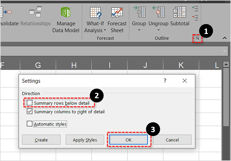
- Go to the “Data” tab.
- In the “Outline” section, click on the arrow icon in the lower right corner.
- This will open the Outline Settings menu.
- Uncheck the box for “Summary rows below detail”.
- Click “OK”.
Notice the change in the grouping levels to the left of column A.
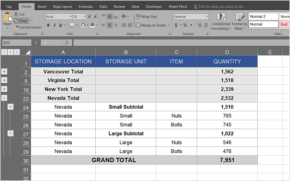
Now that you’ve successfully grouped your data, you can use the “+” and “-“ buttons to show and hide details for each of the groups. To collapse or expand an entire group, simply click on the numbers at the top of the grouping column.
Manual Grouping
Depending on how your data is structured, it may not follow the guidelines presented at the beginning of the previous section. For example, it may contain blank rows or columns as a design feature. That could prevent the auto-grouping option to properly do its magic on the entire sheet.
That’s why Excel allows you to group your data manually as well. You can group just one portion of your sheet and leave the rest ungrouped. Or you may find it important to do the grouping manually, section by section, in order to make sure that the data is ok.
Whatever the reason, just make sure that you don’t have any hidden rows or columns before you proceed. This may interfere with the grouping and leave you with the incorrect figures.
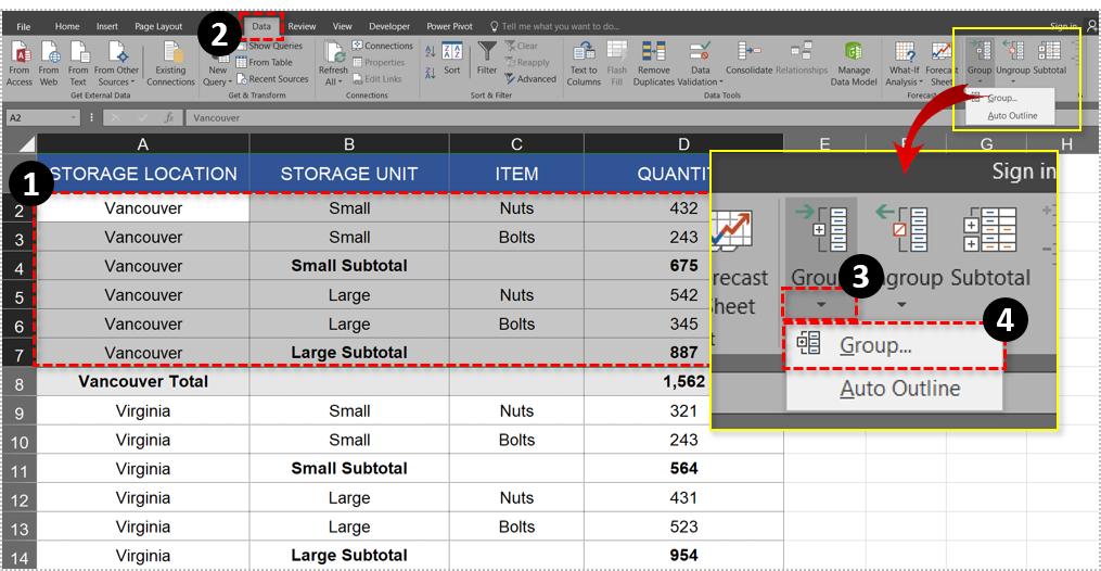
To manually group your data:
- Select the rows you would like to put into a group.
- Go to the “Data” tab.
- In the “Outline” section, click on the “Group” icon. You can also click on the black arrow and select “Group…”.

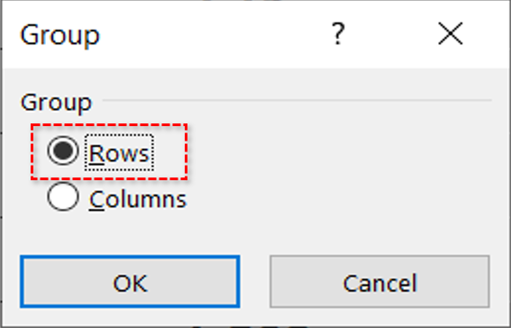
- The “Group” menu appears.
- Select “Rows” and click “OK”.

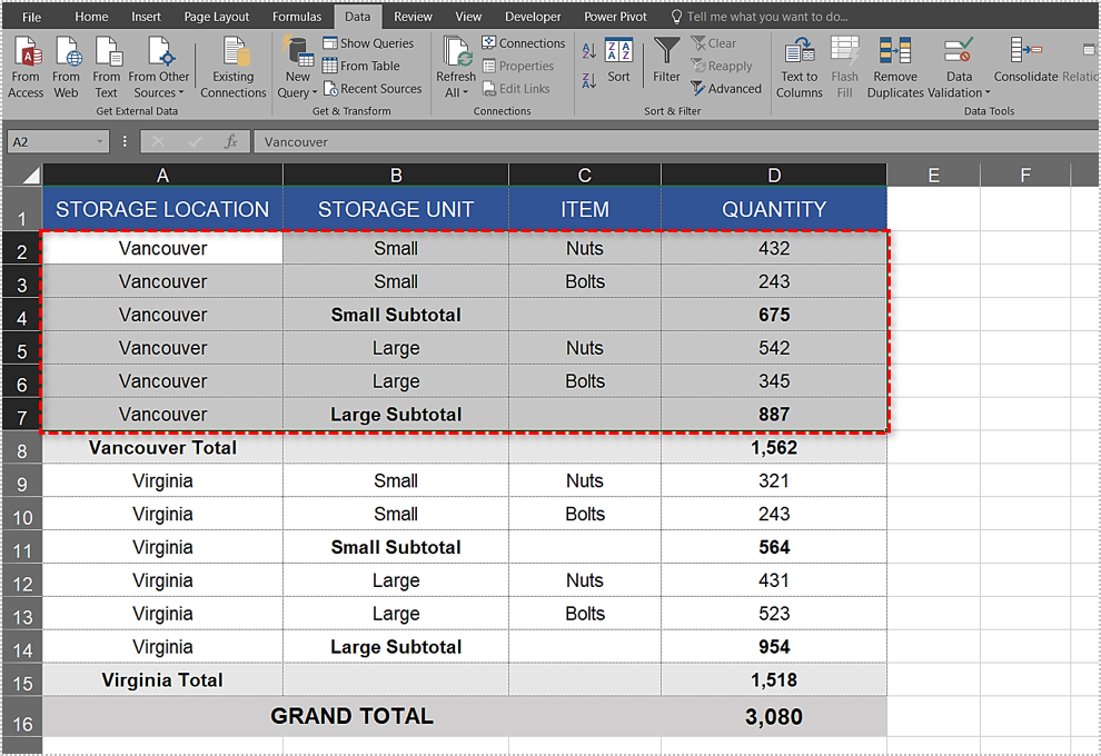
Now that your data is grouped, the group levels will appear to the left of column A.
Choosing What to Group
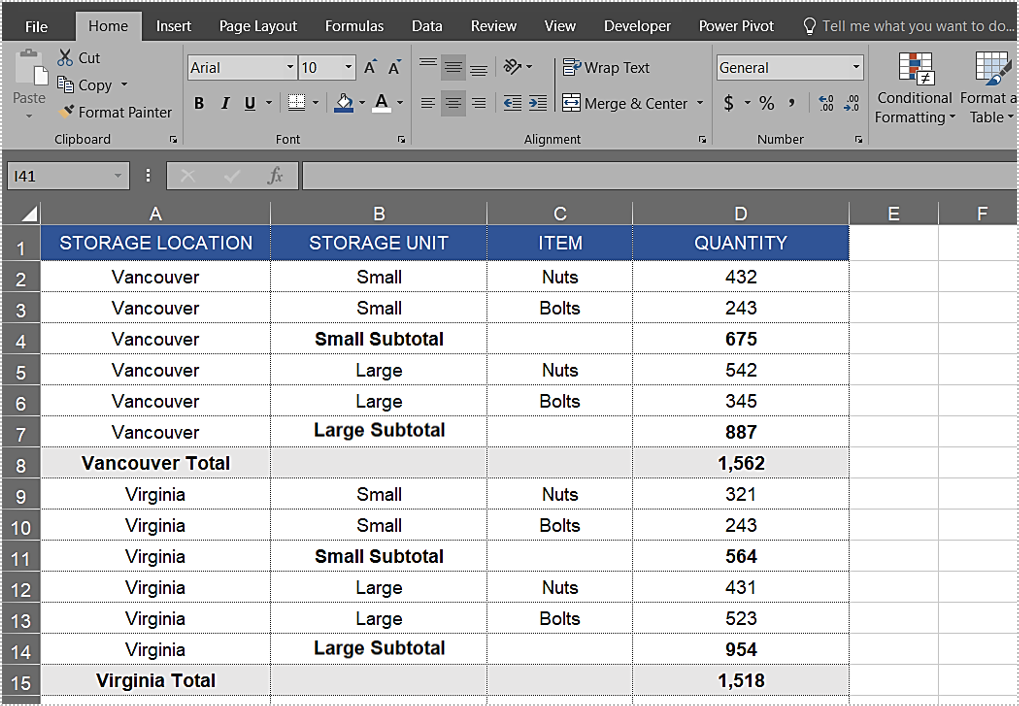
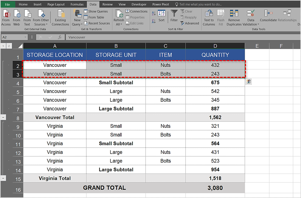
When selecting the subsets you want to group, it is important to know which rows to select and which not to. Looking at the example used in this article, let’s suppose you only want to see how many items are available in Vancouver and Virginia separately.
For Vancouver, first select rows 2 to 7. Then group them manually, as explained in the previous section.
For Virginia, group rows 9 to 14. Now, when you collapse these groups, you will see the sum totals for each of the cities, without having to look at the breakdown figures.
You can group their subsets as well. To see how many items Vancouver’s small storage holds, select rows 2 to 3 and group them. Following this logic, you can group all other subsets in this table.
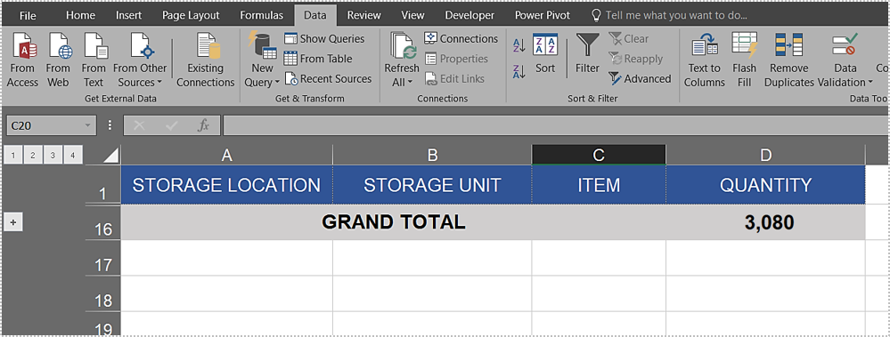
Sometimes, you might want to see how many items are there in total only. And you’re not interested in how they are distributed by city and storage type. To do so, just group rows 2 to 15 and click on number 1 in the grouping column. To see the full breakdown, click on the number 4.
Group Your Data Wisely
The examples in this article mainly explain how to group rows. Clearly, the same principle applies when grouping columns. Now that you know how to group data in Excel, it opens up new ways to further optimize your data analysis.
Is this the first time you learn about how grouping works in Excel? Do you find it useful? If you have any tips on this matter, or any other option in Excel, please share in the comments below.