

How to Change Currency in Google Sheets

Google Sheets is an amazing application used to track and manage financial transactions. It neatly organizes invoices, payments, or investments.
When you start writing numbers in the sheet, by default, they’ll appear as numbers and not currencies. Therefore, you’ll have to make some tweaks, if your work is of a monetary nature. But don’t worry, we’ve got you covered. In this article, you’ll learn how to change the currency in Google Sheets and get the latest exchange rates. Plus, you’ll see how Google Finance formulas can help your business tremendously.
Applying Currency Format
You’ve started typing the numbers you need to track your financial records, and you’re now wondering how to apply the currency format. It really isn’t difficult, just follow these steps:
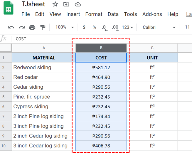
- Select the columns where you want to apply the currency.
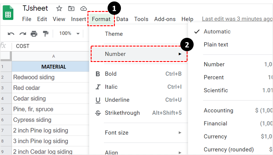
- Now head over to “Format” and click on “Number” from the dropdown menu.
- Here you’ll see different currency options. Tap on “Currency”.

There you go. The numbers in the selected column now show the currency symbol. Most likely it’ll be your country’s default currency. If it’s not, be sure to check out the next section.
Note: You should know that you’ll have to apply this function any time you want to have the currency format, as Google Sheets doesn’t save it automatically.

Changing the Currency
Now, let’s say for some reason the default currency isn’t the one you use in your country – which can sometimes happen. Google Sheets has an option to change this. The steps are as follows:
- Once again, select the column where you want the currency applied.

- Click on “Format” and then on “Number”.

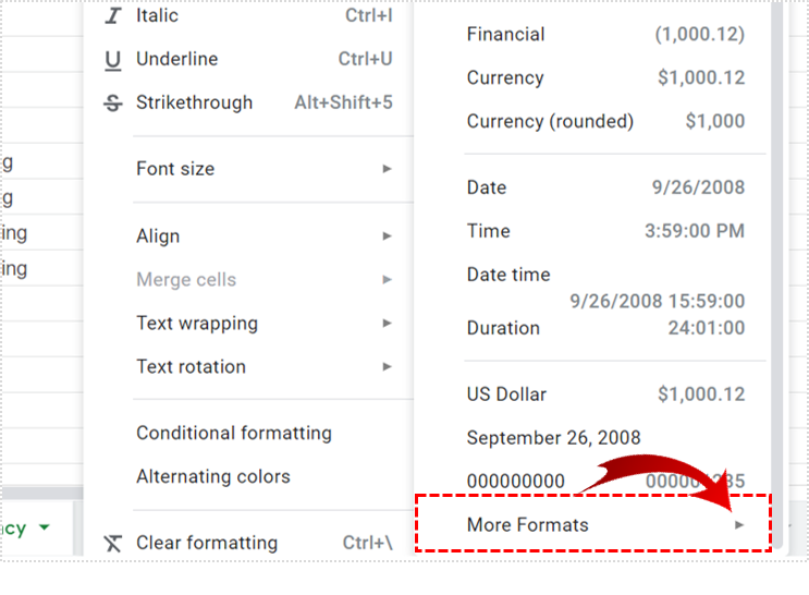
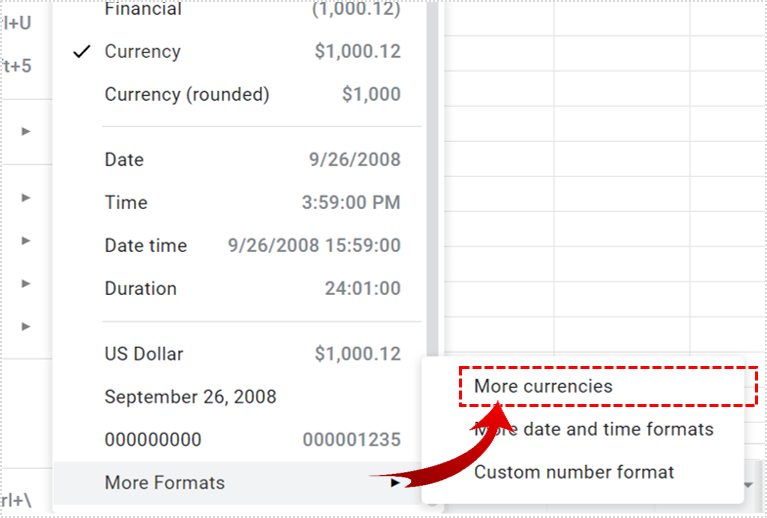
- Scroll down and find “More Formats”. Tap on that.

- Click on “More currencies”.

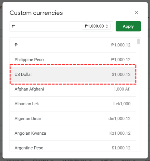
- Here you have a bunch of different currencies, so just select the one you need.

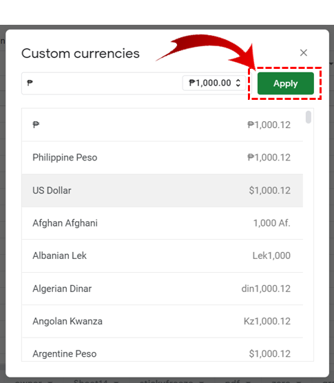
- Finish by clicking on “Apply”.

Automatic Currency Conversion
Google Sheets has done an amazing job adding a lot of currencies as it helps organizations with clients all over the world. Additionally, if you’re someone who saves money in local and foreign values, Google Sheets gives you a clear review of all your savings. But calculating the exchange rates manually can be quite time-consuming. Luckily, Google Sheets has an option for this, too.
Let’s see what you have to do first:
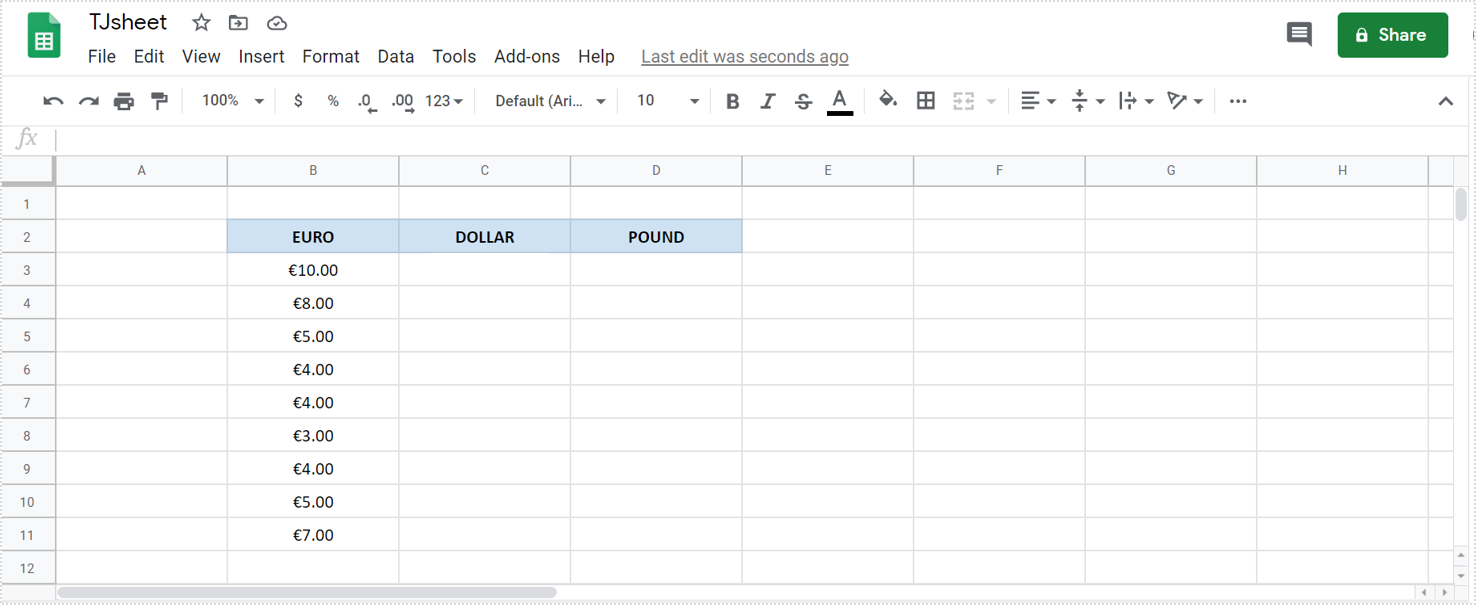
- You should have separate columns for each currency. For example, here you have the euro, dollar, and pound.

- You should now apply the correct currency to each column. Check the previous section on how to add more currencies.
Now, to convert to another currency (in this case dollar and euro), you’ll use the “GoogleFinance” formula:
- Go to the cell where you want the conversion to occur.
- Next, go to the formula bar.
- Now, type the following: “=GoogleFinance(“CURRENCY:EURUSD”).
Check the formula you wrote is the same one you see here. Note that you must have the brackets, the quotation marks and capital letters.
Now that you’ve applied the formula, the value in the selected column will be equal to the currency you wanted to convert from (in this case, the euro). So, from the photo, you can see that $1.20 in the column where we applied the formula. This means that €1 equals $1.20.

However, in order to set the exchange rate, you’ll have to do this too: Simply put the letter representing the original currency column and “*” in front of the formula. Here’s what you’ve got to type:
- In the formula bar, type the following: =B3*GoogleFinance(“CURRENCY:EURUSD”).
- Now drag down and you’ll see the exchange rates.

To change the currency to pounds, you’ll apply the same formula and just change the currency code. In this instance, GBP is the pound’s currency code.
Removing Currency Signs
For people working with monetary data, having currency symbols is a handy thing. However, if you work with data in only one value, the symbol might not be necessary for you.
When you format currencies in Google Sheets, the value sign will always appear before the number. So if you want to learn how to remove it, there is a way. What you’ve got to do is to change the cell formatting since it’s probably set to “Currency” and displaying the currency symbol. Here’s how to do it:
- Select the column where you want to apply this function.
- Head over to “Format” and click on “Number”.
- Now you’ll have to click on “Number” from the dropdown menu, instead of “Currency”.
There you go. Now you’ll just see the numbers in the column.
Explore
If you’re using it for personal reasons, Google Sheets can be a way to track your monthly budget, expenses, salary, etc. Not only can you manage your finances, but you can also do it using different currencies.
Furthermore, if you’re using Google Sheets for your business, you’ll be able to work with multiple currencies and easily convert values. How do you use Google Sheets to manage your finances? Do you use any other Google Finance formulas in Google Sheets? Share your experiences with the community in the comments section below.