

How to Create a Dropdown List in Excel
Dropdown lists can contribute to a much more efficient and effective spreadsheet. The more complex the spreadsheet, the more useful drop down boxes can be. If you’re struggling to create one in your spreadsheet, help is at hand. Here’s how to create a dropdown list in Excel.
There are actually a couple of ways to create a dropdown list in Excel. They both use the same fundamental steps but offer a little flexibility in how you build your list.
Create dropdown lists in Excel
Here is the main way you can create a dropdown list in Excel 2013 onwards. You have to create one sheet to host the data and another sheet to host the spreadsheet itself. For example, you want the dropdown list to appear on Sheet 1 so you will add the data for that box in Sheet 2. This keeps everything separate.
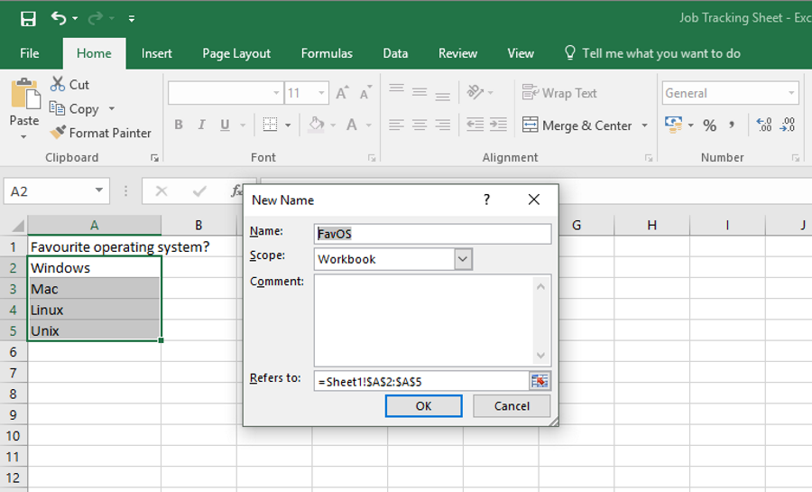
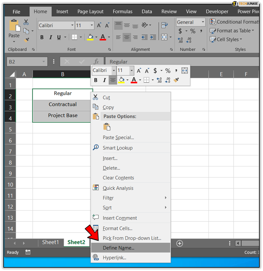
- Type the entries you want to feature in your dropdown in Sheet 2 in Excel.

- Select them all, right click and select ‘Define name’ from the options.

- Name the box and click OK.

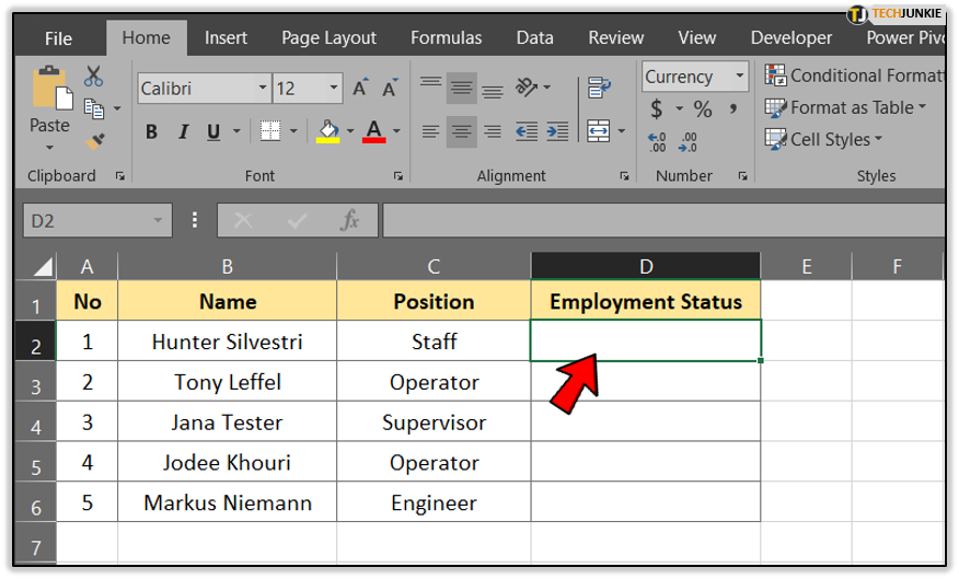
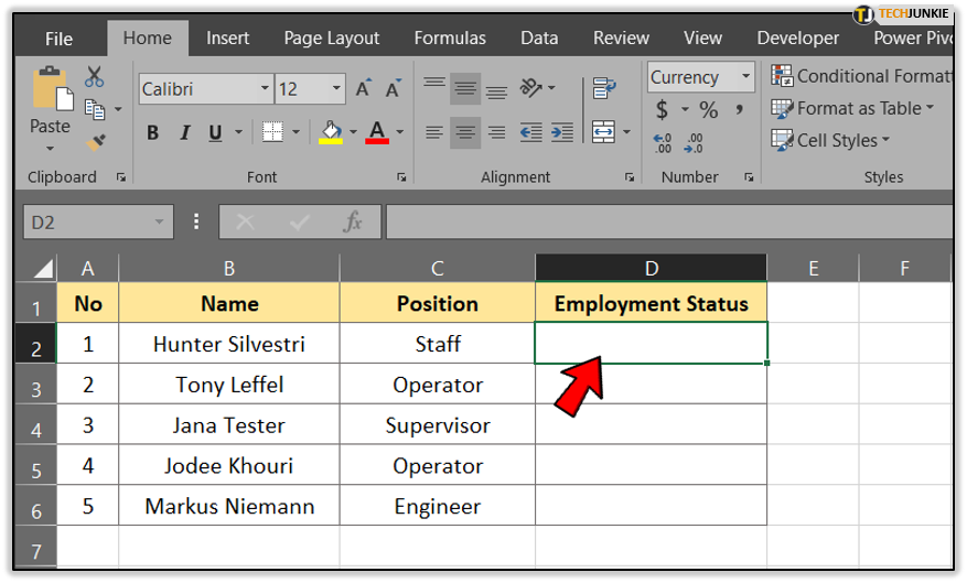
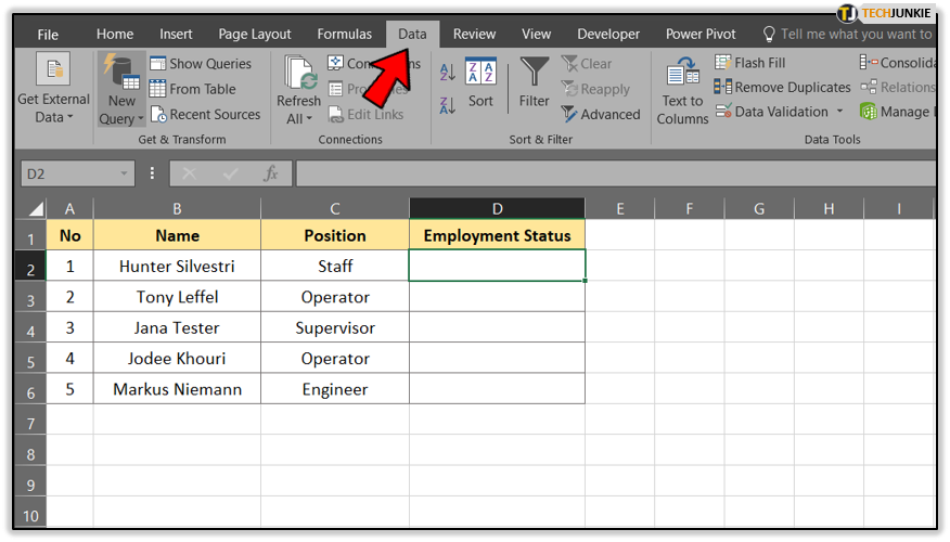
- Click the cell on Sheet 1 in which you want your dropdown box to appear.

- Click the Data tab and Data Validation.

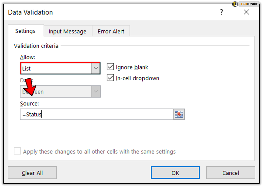
- Select List in the Allow box and type ‘=NAME’ in the Source box. Where you see NAME, add the name you gave in step 3.

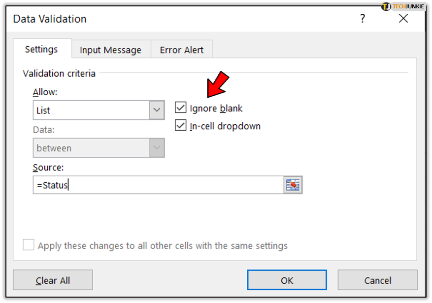
- Select ‘Ignore blank’ and ‘In-cell dropdown’ as you see fit.

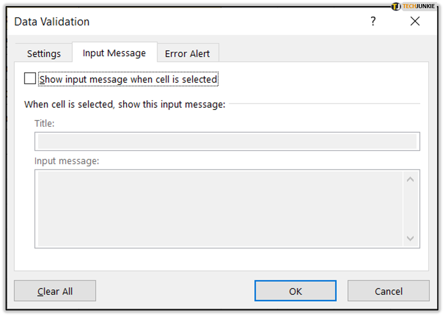
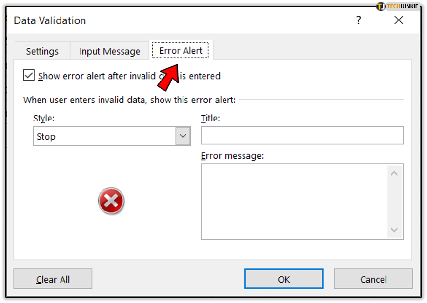
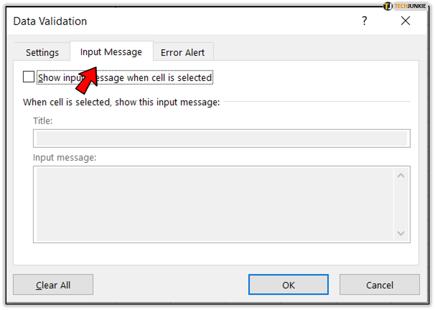
- Click the Input Message tab and either uncheck the box or add a message to be displayed once a selection is made in the dropdown box.

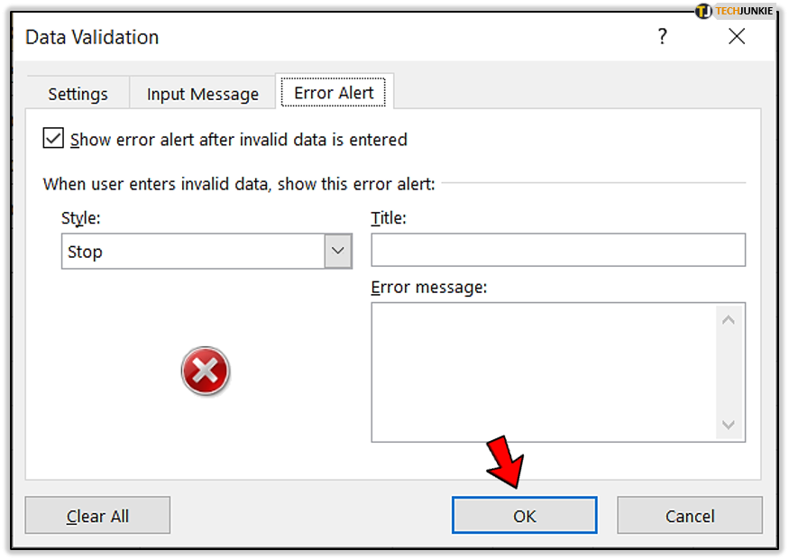
- Click the Error Alert box if you want to make changes.

- Otherwise click OK.


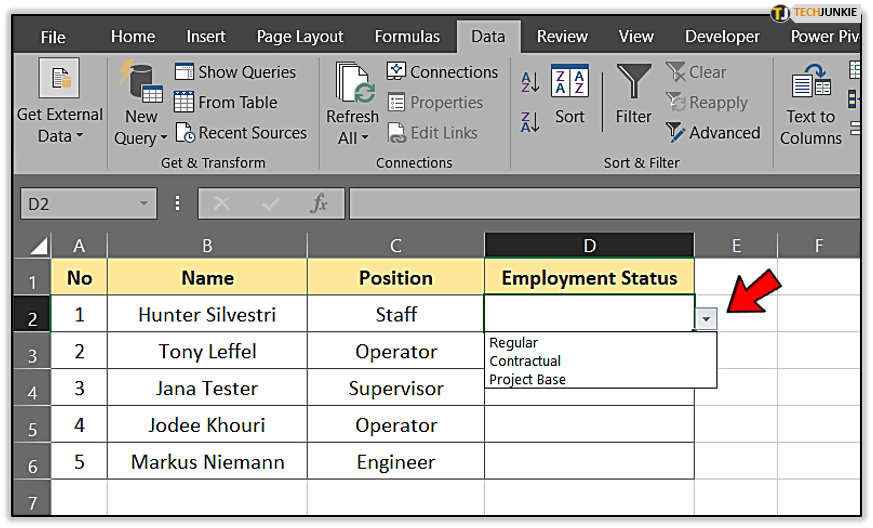
You dropdown list should now appear in the cell you specified. Give it a quick test to make sure it works.
Use a table to populate a dropdown list
You can also select a table to build your list. To use a table in a dropdown list in Excel. By using a table, you are able to make changes on the fly without having to edit the named ranges. If your spreadsheet is always evolving, this could save a lot of time.
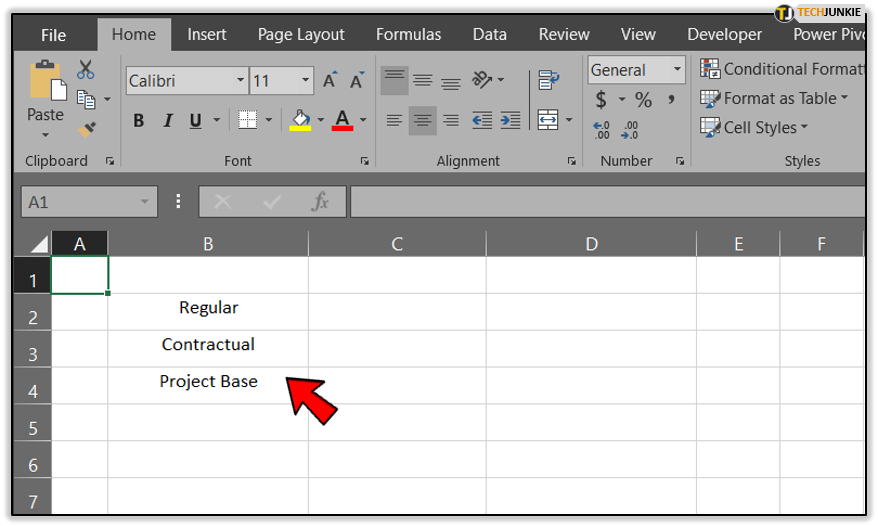
- Type the entries you want to feature in your dropdown in Sheet 2 in Excel.
- Highlight the entries, click the Insert tab and then Table. Define the table and name it.

- Click the cell on Sheet 1 in which you want your dropdown box to appear.

- Click the Data tab and Data Validation.

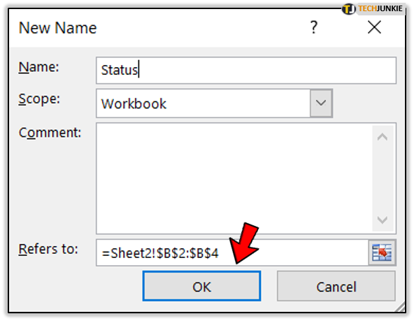
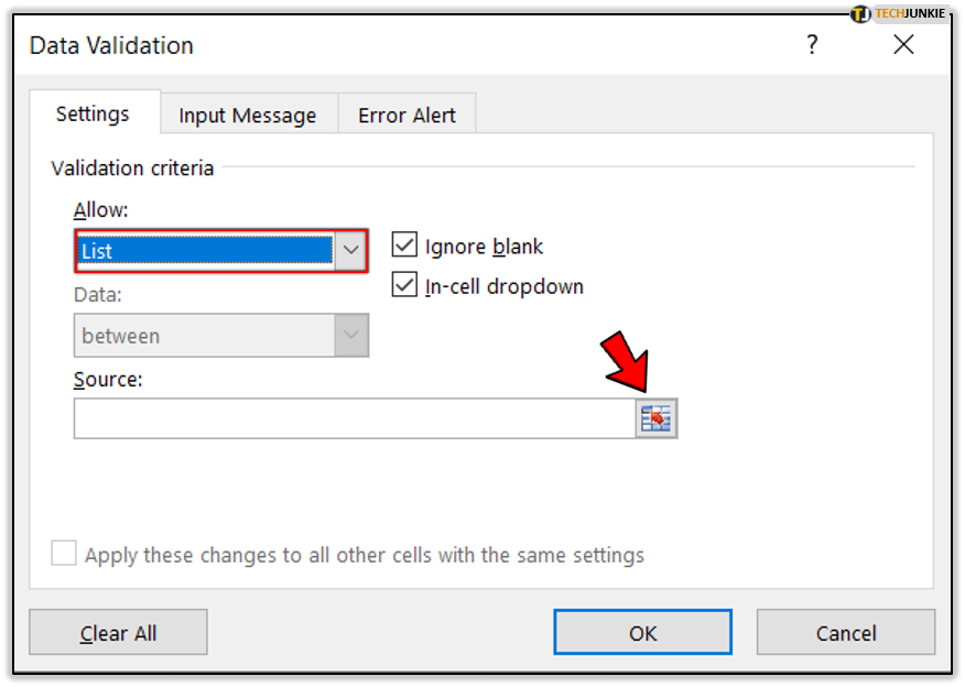
- Select List in the Allow box and click the little cell icon next to the Source box.

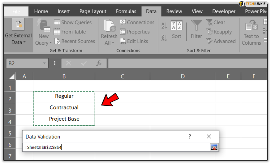
- Highlight the cells in the table you want to feature in the dropdown box. The Source box should then read something like ‘‘=Sheet2!$B$2:$B$4’.
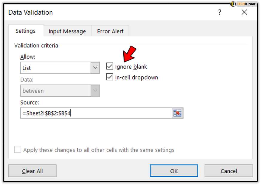
- Select ‘Ignore blank’ and ‘In-cell dropdown’ as you see fit.

- Click the Input Message tab and either uncheck the box or add a message to be displayed once a selection is made in the dropdown box.

- Click the Error Alert box if you want to make changes.
- Otherwise click OK.


The new dropdown box should appear in the cell on Sheet 1 where you selected.
That’s it. Now you have a fully functional dropdown list in Excel!