How to Paste Link and Transpose Functions in Excel

The link and transpose functions in Excel are mutually exclusive. This means that transposed cells won’t work as links on your sheet. In other words, any changes that you make to the original cells are not reflected in the transposed copy.

However, your projects often require you to both transpose and link the cells/column. So is there a way to utilize both functions? Of course there is, and we’ll present you with four different methods to do it.

It is safe to say that these tricks are part of intermediate Excel knowledge, but if you follow the steps to a T, there won’t be any trial and error even if you are a complete novice.

The Pasting Problem

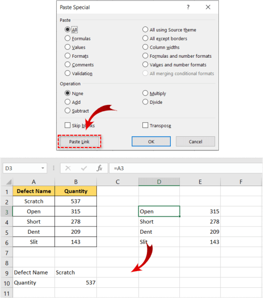
For the purposes of this article, let’s assume you want to transpose columns into the same sheet. So what do you do? Select the columns, hit Ctrl + C (Cmd + C on a Mac), and choose the paste destination. Then, click the Paste options, select Paste Special, and tick the box in front of Transpose.

But as soon as you tick the box, Paste Link gets grayed out. Luckily, there are some formulas and tricks that help you work around this issue. Let’s take a look at them.

TRANSPOSE – Array Formula

The main advantage of this formula is that you don’t need to manually drag and drop the cells. However, it does come with certain downsides. For example, the size is not easy to change, which means that you need to use the formula again if the source cell range changes.

Similar issues apply to other array formulas, though, and this one helps you solve the link-transpose problem fairly quickly.

Step 1

Copy the cells and click on the top-left cell in the area you wish to paste the cells to. Press Ctrl + Alt + V to access the Paste Special window. You can also do it from the Excel toolbar.

Step 2

Once you access the window, tick Formats under Paste, choose Transpose at the bottom-right, and click OK. This action only transposes the formatting, not the values, and there are two reasons you need to do this. First, you’ll know the transposed cells range. Second, you retain the original cells’ format.

Step 3

The entire pasting area needs to be selected and you can do this after you paste formats. Now, type =TRANSPOSE (‘Original Range’) and hit Ctrl + Shift + Enter.

Note: It’s important to press Enter together with Ctrl and Shift. Otherwise, the program doesn’t recognize the command correctly and it automatically generates curly brackets.

Link and Transpose – Manual Method

Yes, Excel is all about automation and using functions to make cell and column manipulation easier. However, if you are dealing with a fairly small cell range, manual link and transpose is often the quickest solution. Admittedly, though, there is room for error if you are not careful enough.

Step 1

Select your cells and copy/paste them using the Paste Special option. This time, you don’t tick the box in front of Transpose and you leave options under Paste as default.

Step 2

Click the Paste Link button at the bottom-left and your data will be pasted in the form of links.

Step 3

Here comes the hard part. You need to manually drag then drop cells into the new area. At the same time, you need to be careful to exchange rows and columns.

OFFSET Formula

This is one of the most powerful tools to paste cells, link, and transpose them. However, it might not be easy if you are new to Excel, so we will try to make the steps as clear as possible.

Step 1

You need to prepare the numbers on the left and on the top. For example, if there are three rows, you’ll use 0-2, and if there are two columns, you’ll use 0-1. The method is the total number of rows and columns minus 1.

Step 2

Next, you need to find and define the base cell. This cell should stay intact when you copy/paste and this is why you use special symbols for the cell. Let’s say the base cell is B2: you’ll need to insert the dollar sign to single out this cell. It should look like this within the formula: =OFFSET($B$2.

Step 3

Now, you need to define the distance (in rows) between the base cell and target cell. This number needs to increase when you move the formula to the right. For this reason, there shouldn’t be any dollar sign in front of the function column. Instead, the first row gets fixed with the dollar sign.

For example, if the function is in column F, the function should look like this: =OFFSET($B$2, F$1.

Step 4

Like rows, columns also need to increase after you link and transpose. You also use the dollar sign to fix one column but allow the rows to increase. To make this clear, it is best to refer to the example which may look like this: =OFFSET($B$2, F$1, $E2).

How to Excel at Excel

Besides the given method there are also third-party tools you can use to link and transpose. And if the given methods don’t yield satisfactory results, it might be best to use one such tool.

Have you used one of those transpose/link apps to perform this operation in Excel? Were you satisfied with the result? Share your experiences in the comments section below.