

Get More Out of Google Sheets With Conditional Formatting
If you work with data a lot, you will likely spend as much time making your spreadsheet look good and make sense as you will creating the sheet in the first place. You can automate a lot of that with conditional formatting. Along with some custom formulas, you can create fantastic looking spreadsheets in half the time. Here’s how.
Conditional formatting tells a spreadsheet that if a cell contains X to do Y. So if a cell contains a specific data element, it is to format it in a certain way and if it doesn’t contain that data, to format it in a different way. This makes it easy to identify specific data points and get the system to do some of the work instead of you doing it manually.
The learning curve isn’t as steep as you might think either, which is ideal for me as I’m not exactly a master at Google Sheets. Nevertheless, I use conditional formatting a lot when presenting data.
Conditional formatting in Google Sheets
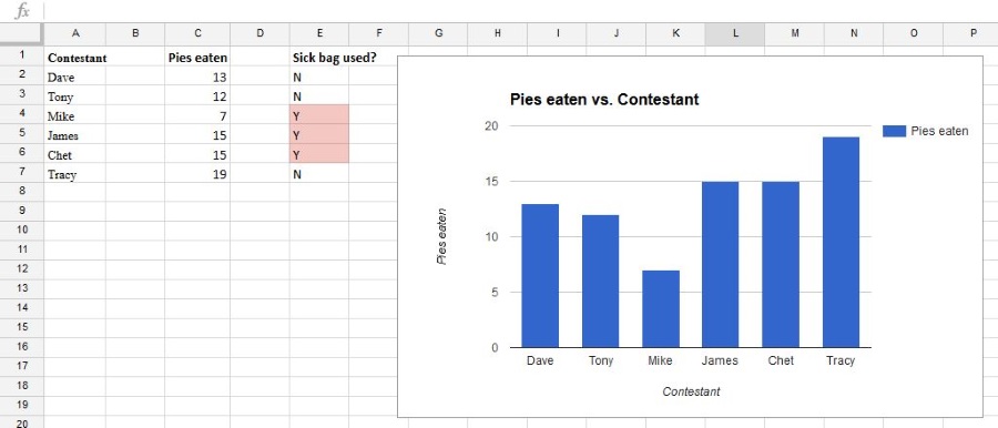
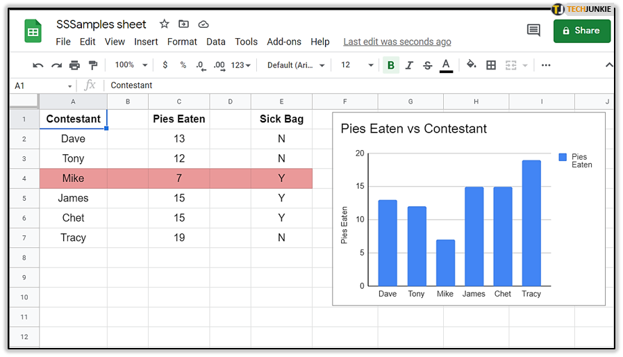
I’m going to use a fake spreadsheet of a pie eating contest. It’s the same one I used in ‘How to build graphs in Google Sheets’ so if you read that, it should be recognizable. It doesn’t matter if you haven’t seen it before as it isn’t exactly difficult to grasp.
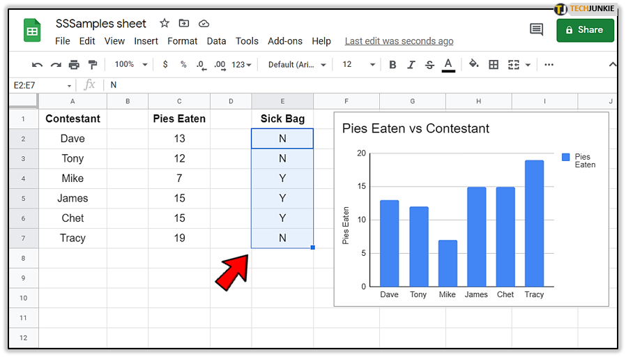
To make conditional formatting work, I have added an extra column with a simple Yes or No entry. It is this column that I will format. It obviously doesn’t have to be as simple as that but for the purposes of this tutorial works well enough.
- Open your sheet and select the range of data you want to use.

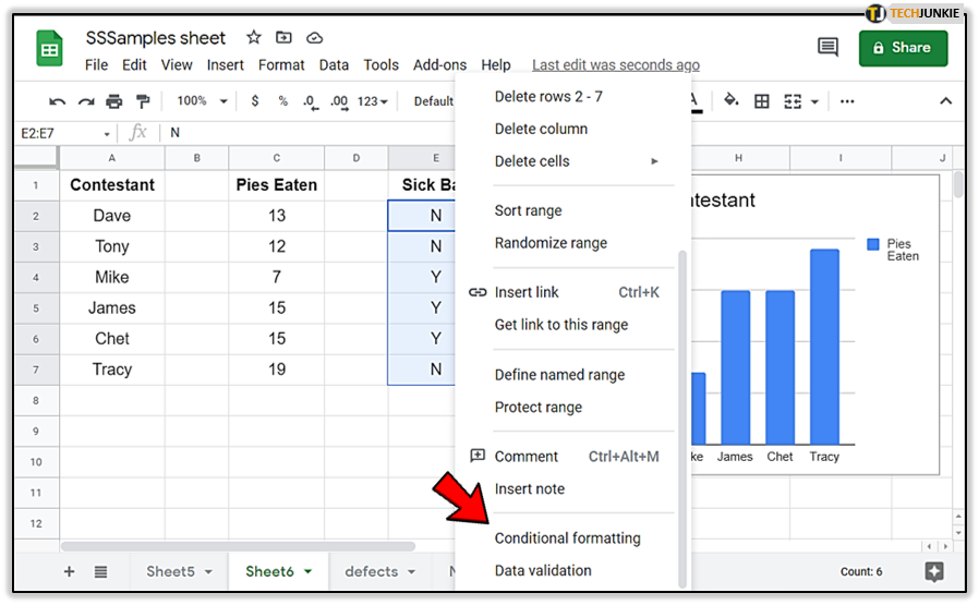
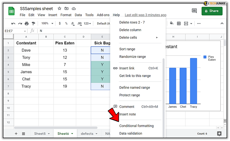
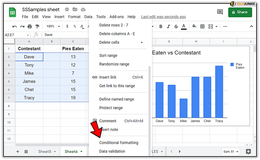
- Right click and select Conditional formatting.

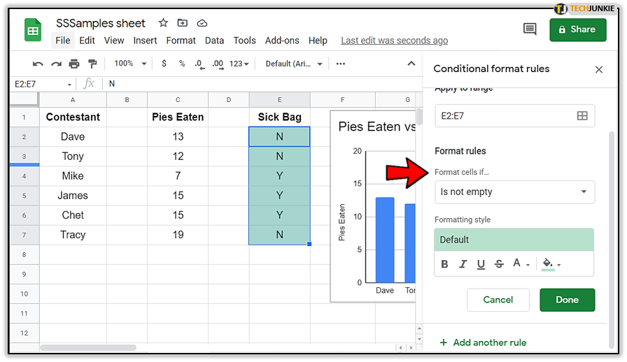
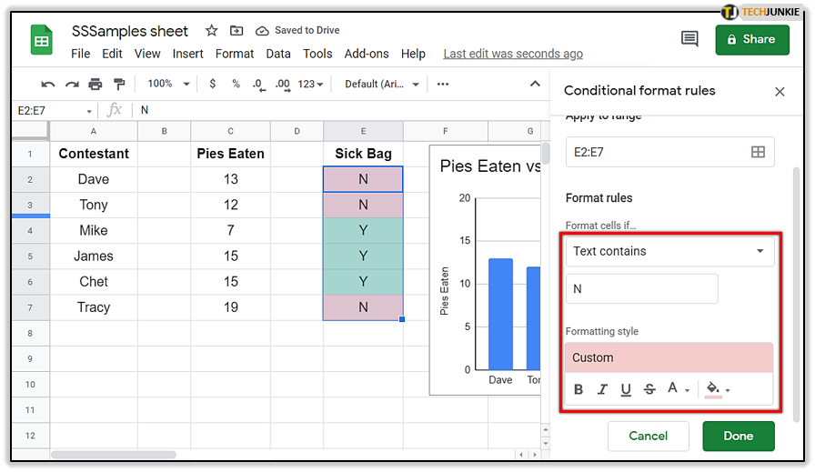
- Select Format cells if… in the new box that appears on the right.

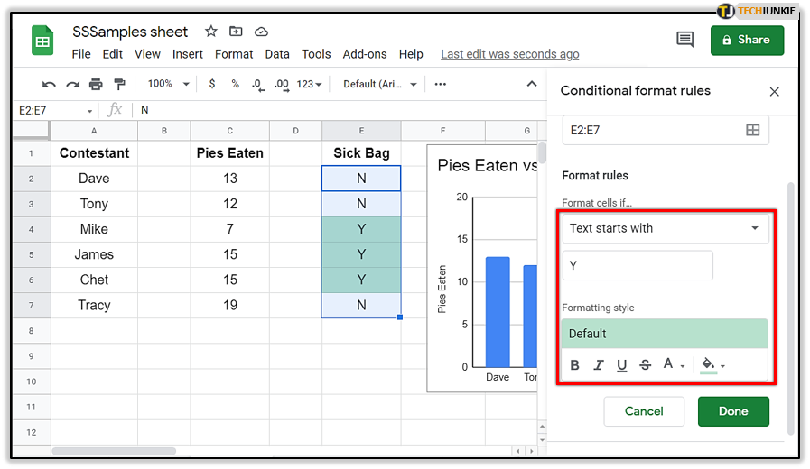
- Select a data point to format and the format you want it to apply.

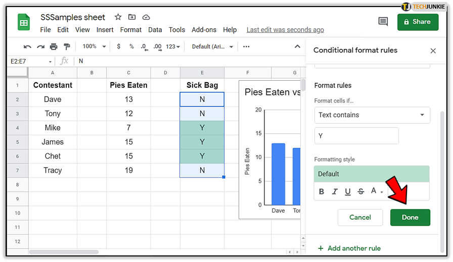
- Select Done.

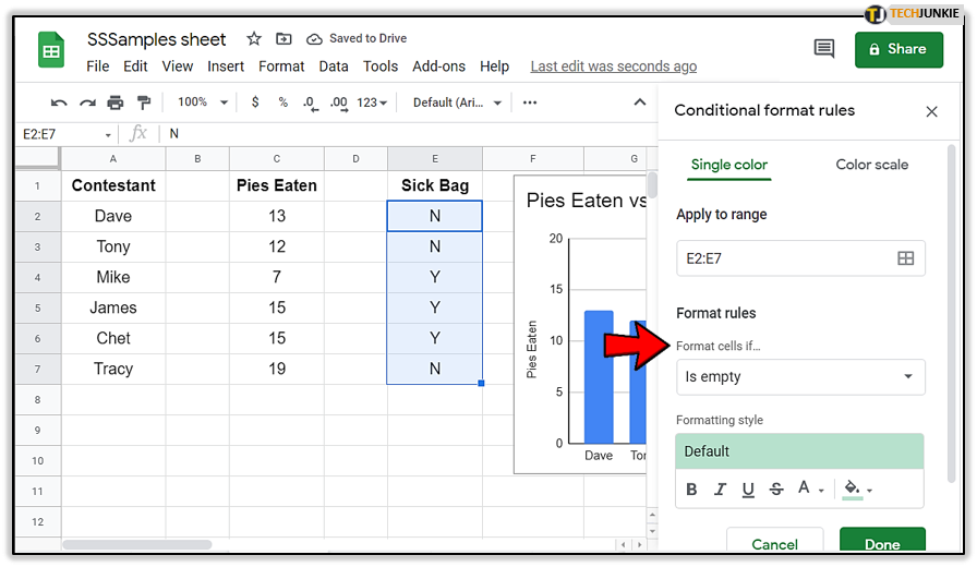
You have a range of conditions you can apply to conditional formatting including empty cells, cells containing a specific character, starts with, ends with, date is, date before, data is less than, equal to or greater than and a whole lot more. There is every conceivable condition here so something should match your needs.
Add more conditions
Once you have set one conditional format you may find one isn’t enough. Fortunately, you can add as many as you like to Google Sheets.
- Open your sheet and select the range of data you just modified.

- Right click and select Conditional formatting.

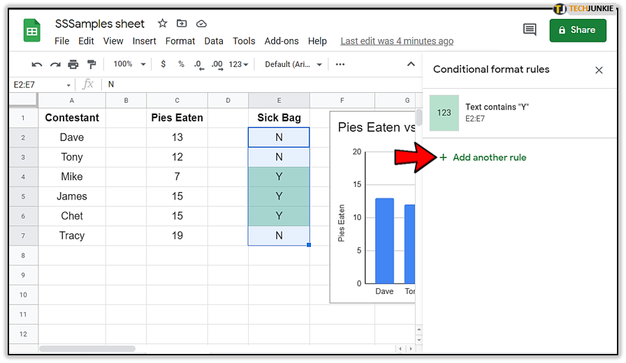
- Select Add another rule at the bottom of the new window.
- Select Format cells if… in the new box that appears on the right.

- Select a data point to format and the format you want it to apply.
- Select Done.
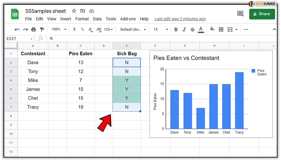
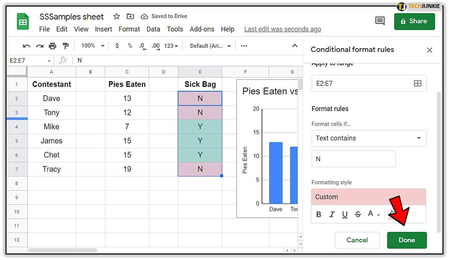
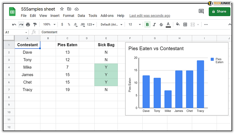
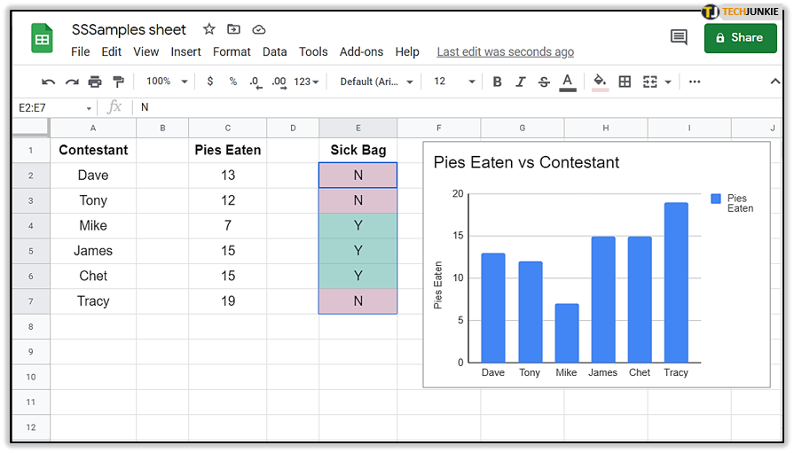
You can rinse and repeat this as many times as you like. In the example, the first formatting I applied was to color green the condition Y under ‘sick bag’. The additional condition I added was to color red N under the same column.
You can go further than just coloring cells. By using custom formula, you can add even more customization to Google Sheets.
Use custom formula to take conditional formatting further
In the above example, I used conditional formatting to color cells to highlight data. What about if you want to color a row containing lots of different data? That’s where custom formulas come in.
- Select all the data you want to include in the formula.

- Right click and select Conditional formatting.

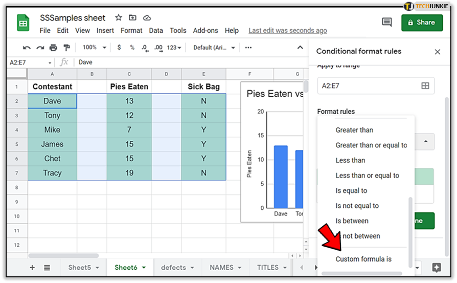
- Select Custom formula is in the new box that appears on the right.

- Enter ‘=$C2<10’ into the empty box and select a formatting style.

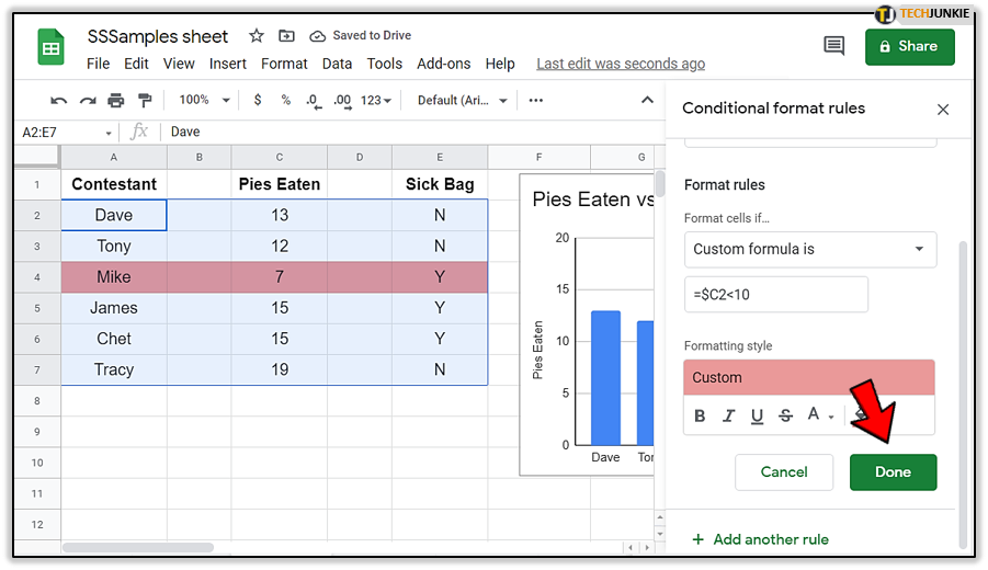
- Select Done.

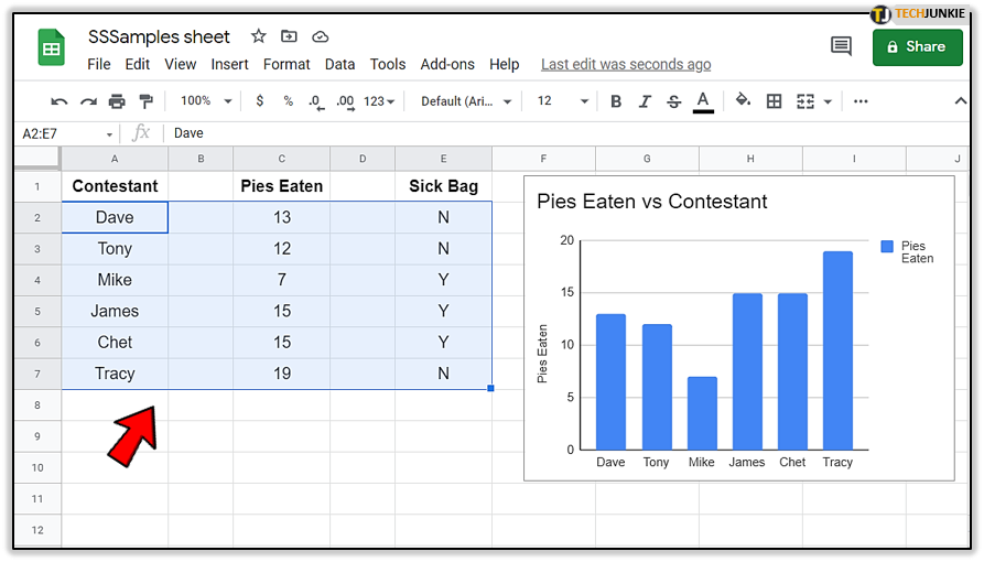
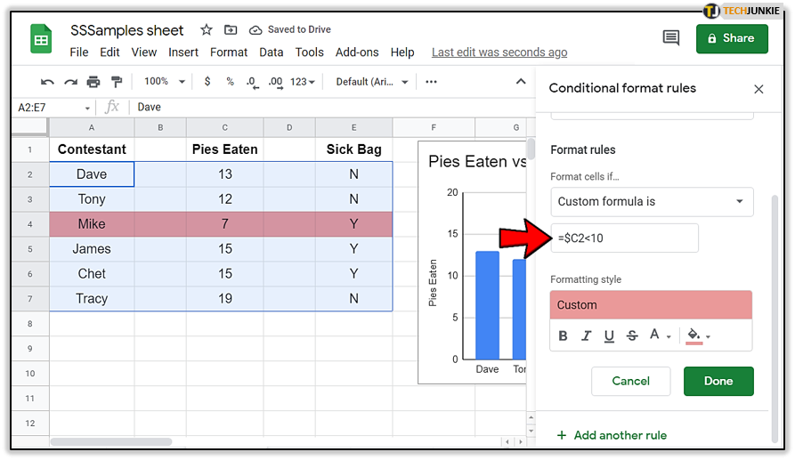
You will see from the image, only the row with the contestant who ate less than 10 pies is highlighted in red. Only one row failed the condition so only one row was formatted according to that formula.
The formula you enter will differ depending on your sheet. Adding ‘=$’ tells Sheets I am adding a formula. Adding ‘C2’ tells it what column and row to use. Using ‘<10’ sets the condition at less than 10. You can use these building blocks to build your own custom formula to set the conditional formatting as you need it.
Like with conditional formatting, you can add as many custom formula as you need to provide the formatting your Sheet requires. It is a very powerful tool and I have only just scratched the surface of its potential here.