

How to Hide Cells in Microsoft Excel

Microsoft Excel is a very popular spreadsheet program because it’s very powerful, yet simple to use. When it comes to tables, there’s hardly anything you can’t do. If you want to hide a certain cell to protect valuable information or to prevent it from distracting you, you can do in no time.
Actually, there are many ways to hide a cell. You can hide rows, columns, or even hide certain cells’ data and still be able to use them in formulas. Read on to master the principles of cell hiding.
Hide Cell Data
If you’d like to hide the data of a single cell, but would prefer the cell to remain visible, you can do this by formatting it.
- Select the cell. This method works for single cells, multiple cells, and entire rows and columns.

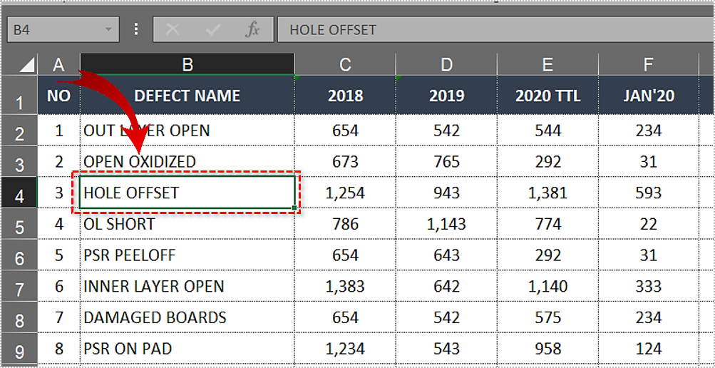
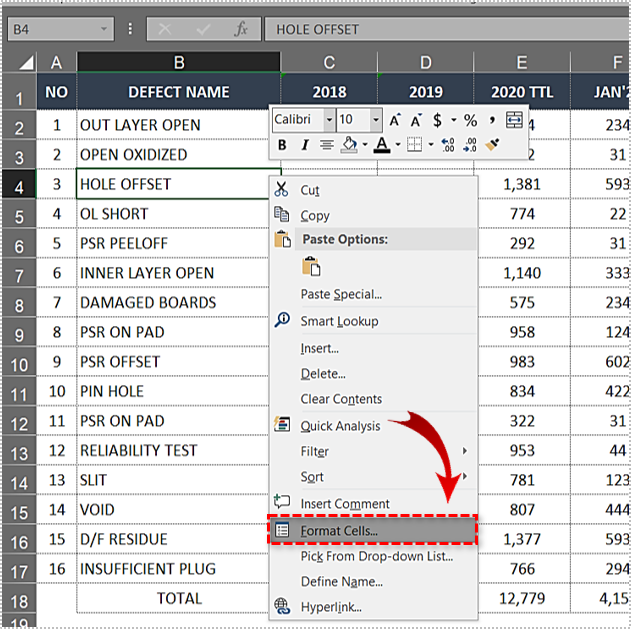
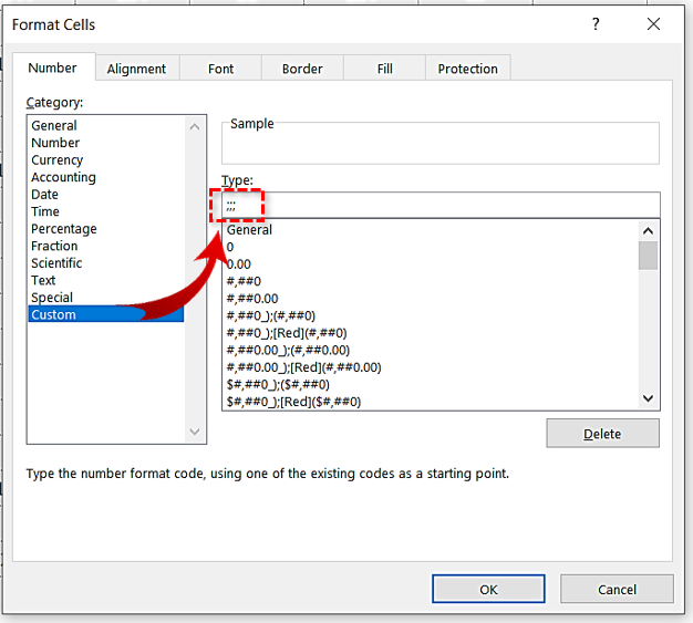
- Right-click on one of the selected cells and choose “Format Cells…”

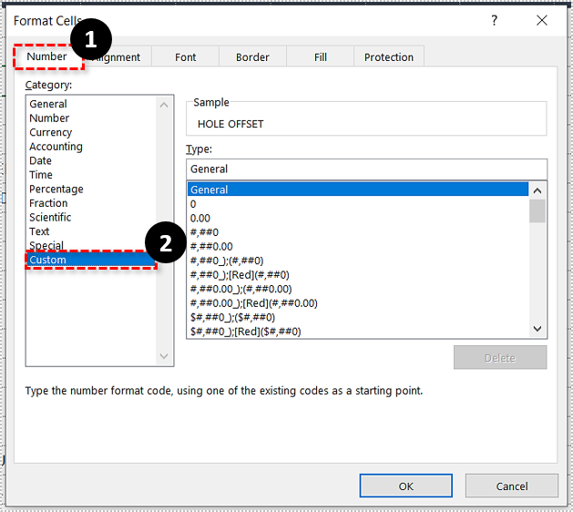
- In the “Format Cells” window that appears, the “Number” tab will already be selected. In its “Category” section to the left, move from “General” to “Custom.”

- Change its type in the “Type” section from “General” to “;;;” (three semicolons).

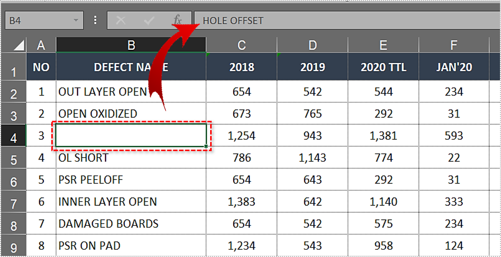
- Click on the “OK” button to save the changes. The formatted cells should show no data, but once selected, you should be able to see their values in the Formula Bar.

Hide and Unhide Rows and Columns Using Ctrl and Shift
The easiest way to hide specific rows and columns is by holding down the Control key to select them one by one. You can also select one row or column, hold Shift, and select another one. This will hide the selected rows or columns as well as the ones between them.
When you’re done selecting rows and columns, right-click on a selected row’s number or column letter and select “Hide.” Excel will let you know you’ve hidden them by marking the place wherever there is a hidden row or column.
To unhide the column D, for example, you need to select columns C and E together, right-click on either column’s letter, and click on “Unhide.” The easiest way to unhide all rows and columns is pressing Ctrl + A to select all of them, right-click on any row or column, and also click on “Unhide.”
Hide Rows, Columns, and Sheets
The Format menu lets you hide and unhide rows, columns, and sheets with a single click.
- In the “Home” tab on top of the window, find the “Cells” category and click on “Format.” This will open a dropdown menu.
- Go to “Hide & Unhide” and see if you want to hide a row, column, or sheet. Naturally, hiding any of these with just a single cell selected hides the entire row or column that contains this cell.
Note: The unhide actions reveal all previously hidden rows, columns, and sheets.
Unhide a Single Row or Column
There’s also a way to unhide a single row or column in Excel. However, you first need to access the row or column that’s hidden.
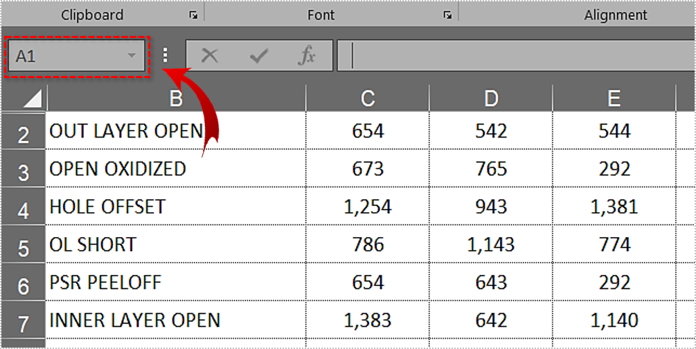
To do this, type a cell’s location in the Name Box. For example, if you want to unhide both the first row and the first column, enter “A1.”
Finally, press Ctrl + Shift + 9 to unhide a row or Ctrl + Shift + 0 to unhide a column. Likewise, Ctrl + 9 hides a row, and Ctrl + 0 hides a column.
Filtering the Info
The great thing about Excel’s cell hiding capabilities is that you have many methods and routes at your disposal. Not only can you hide cells, but you can also hide rows, columns, and entire sheets. Different people have different approaches to hiding cells, so make sure to find out which suits you best.
Why do you want to hide certain cells? Does it improve your workflow? Do you want to hide sensitive info from the prying eyes? Let us know in the comments below.