

How to Group by Date in Google Sheets

Google Sheets is the most convenient way to input data for businesses, organizations, or even personal hobbies. However, certain sheets require you to input lots of data which should really be merged into larger groups.
This is especially useful when these values include dates – you may want to group certain items on a weekly, monthly, or annual basis.
Fortunately, Google Sheets supports this thanks to the recently released ‘Pivot Table’ feature. This article will explain how to group by date using this tool.
Step 1: Preparing a Sheet for Grouping by Date
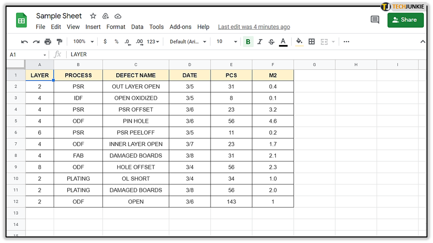
To successfully group by date, you must input the data appropriately. A sheet with clearly written dates will be easy to group in a wide range of different time periods.
Regardless of the purpose and type of your sheet, it’s always important to have one separated column reserved exclusively for dates.
For example, a default business sheet usually has a ‘Date’ column next to ‘Income’ and ‘Expenses.’ This column’s purpose is to show the time period (usually a day, week, month or year) during which income was earned or money spent.
The values in this column should follow the format that you’ve set for dates. Otherwise, Sheets won’t recognize that it’s working with the dates and won’t group the values accordingly. The default date format is MM/DD/YYYY, but you can change this if you want. To do so, follow these steps:
- Open Google Sheets.

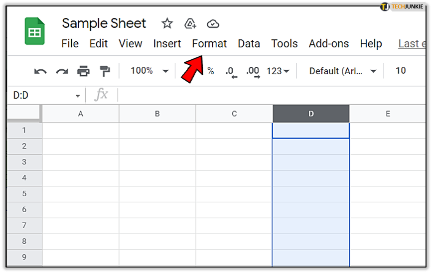
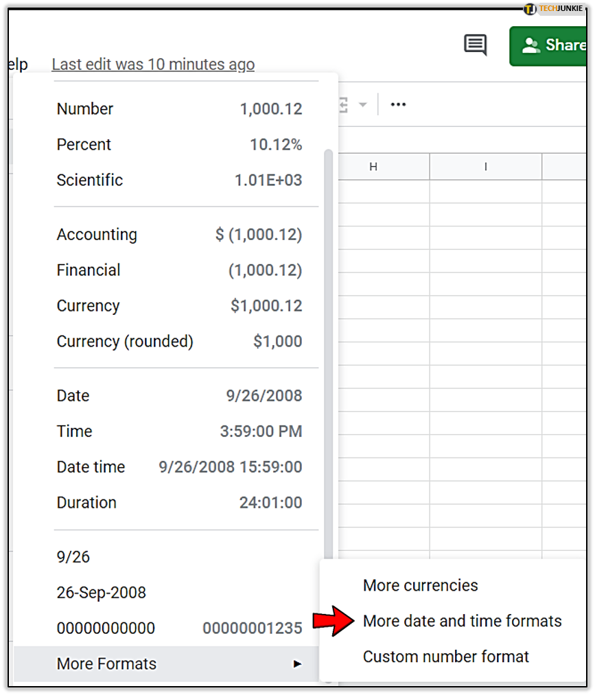
- Click the ‘Format’ option at the top of the page.

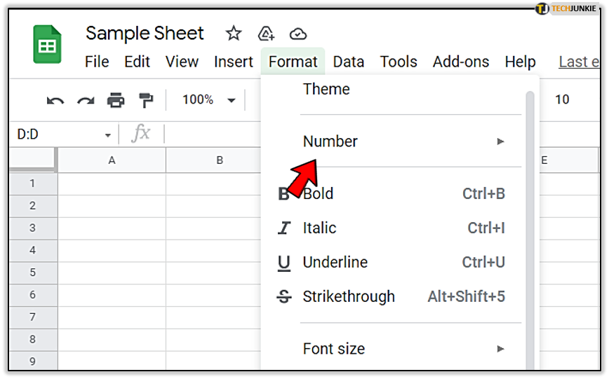
- Hover your mouse over ‘Number.’ A new menu will appear.

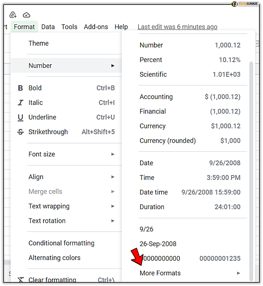
- Do the same over ‘More formats.’

- Click on ‘More date and time formats.’ Here you can choose the date format that you prefer.


When you’ve selected your preferred date format and filled in the sheet with all the necessary data, you can go ahead and make a pivot table.
Step 2: Creating a Pivot Table
The ‘Pivot Table’ feature is the best way to sort and group all the data from your sheet. It’s not only convenient for sorting dates, but also for totaling earnings for a certain period, adding percentages, and various other functions.
To create a pivot table, do the following:
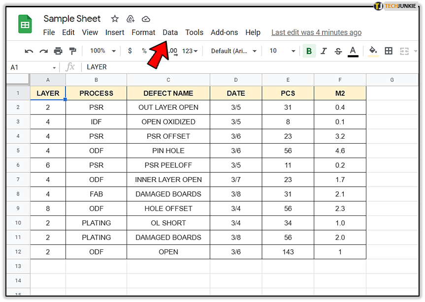
- Open your Google Spreadsheet.

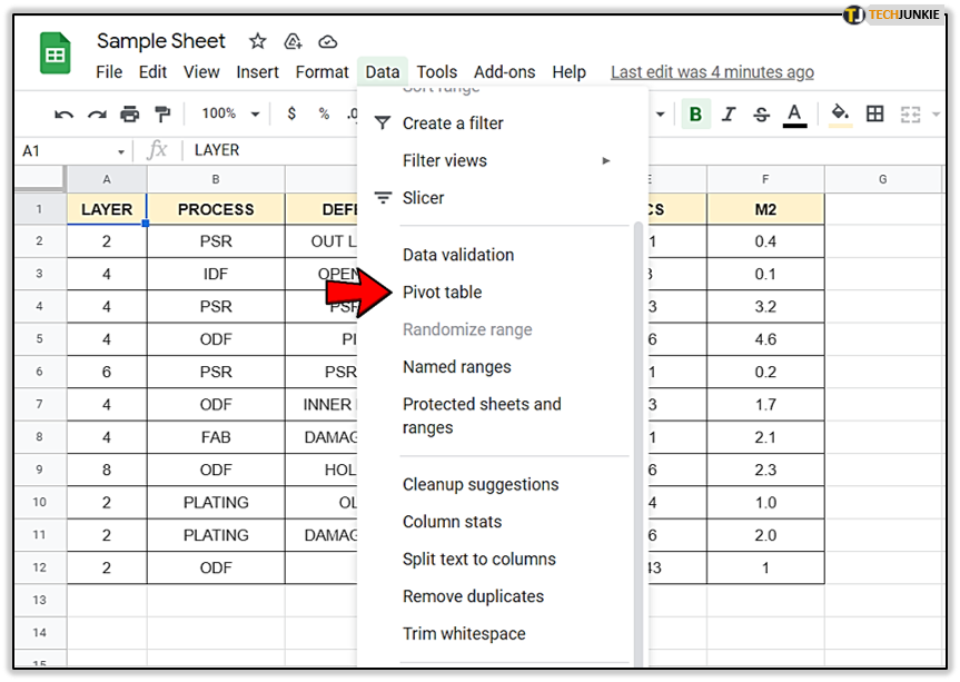
- Click the ‘Data’ bar at the top of the screen.

- Select ‘Pivot Table.’

When you select the Pivot Table option, Sheets will offer you two options – to create a new sheet or create on an existing sheet. It’s recommended to use the new sheet due to clarity. You can easily maneuver between the two using the bottom tabs.
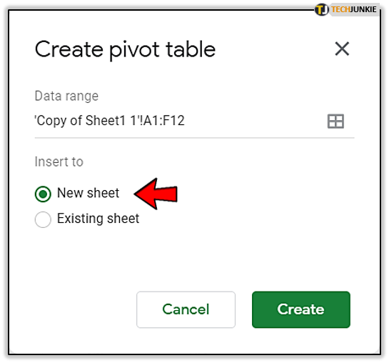
Click the ‘Create’ option to finalize making the ‘Pivot Table.’ You’ll see a griddles sheet with ‘Rows,’ ‘Columns,’ and ‘Values.’ written. This is where the ‘Dates’ column becomes important.
Step 3: Using the Pivot Table Editor to Add Dates
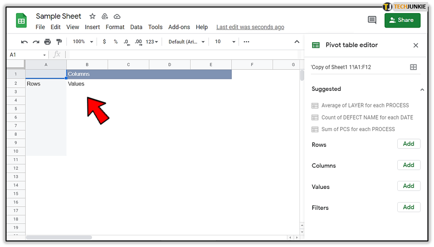
On the right side of the screen, you’ll see a box named ‘Pivot table editor.’ With the help of this box, you can add the values from the previous sheet into your pivot table. Let’s add the ‘Dates’ column:
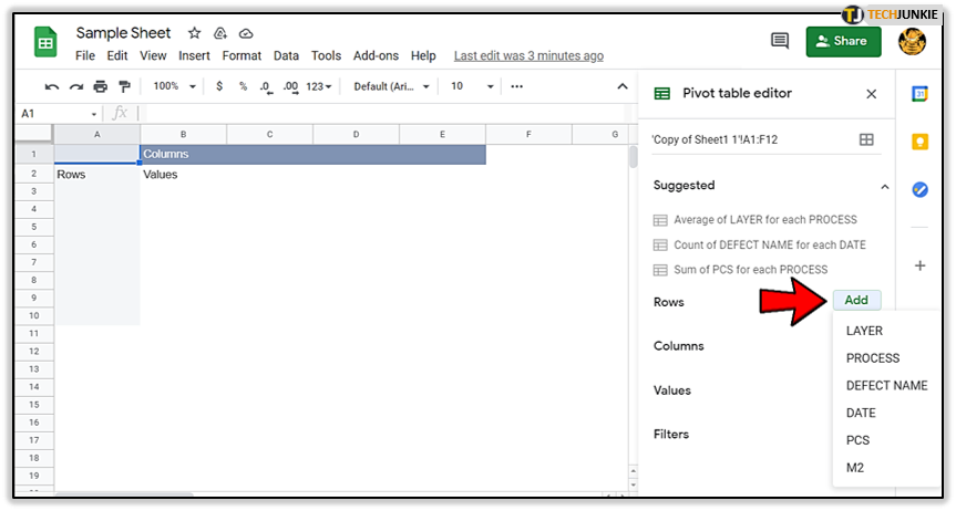
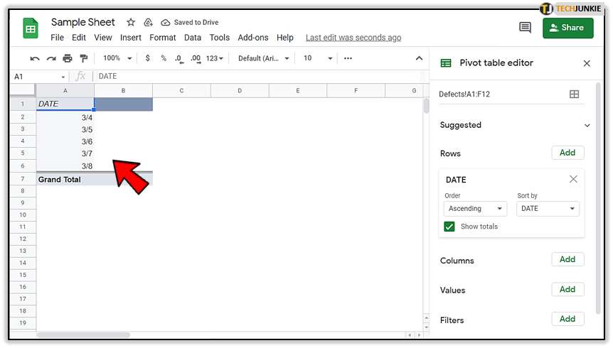
- Click the ‘Add’ button next to the ‘Rows’ in the editor. A dropdown menu will appear displaying all the column headers that you’ve written in the A1, B1, C1 sections (for example ‘Date,’ ‘Process,’ ‘Defect Name,’ etc.

- Select ‘Date.’ (or however you named the column with the dates)

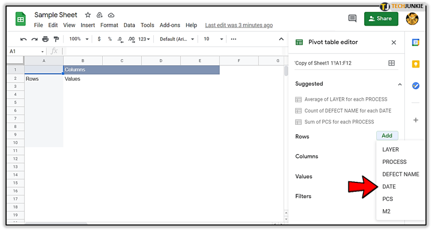
The dates should appear in your pivot table, only not as a group.
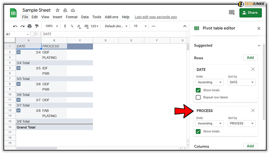
If you want, you can do the same for the other column headers. Just follow the same steps and select each row that you want to list on your pivot table.
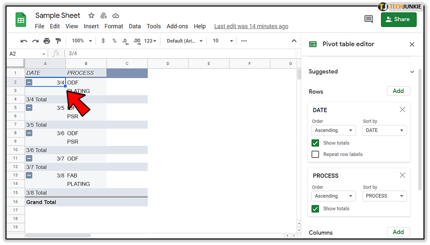
Once you add the dates to your pivot table it’s finally time to group them.
Step 4: Group by Date
When you prepare everything on the pivot table, grouping the values by date is an easy task.
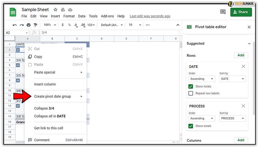
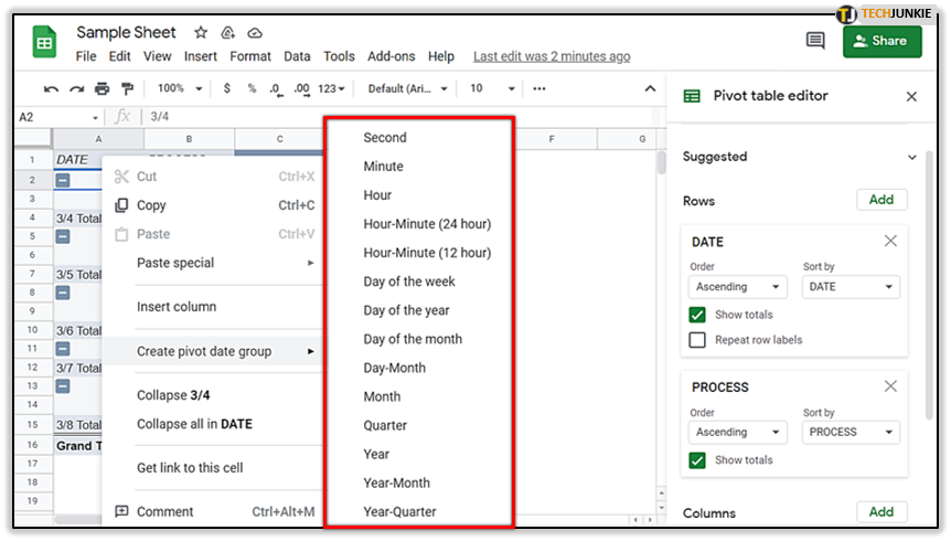
- Right-click on any date in the column.

- Hover your mouse over ‘Create pivot date group.’

- Select the period to group your dates. The dates will group accordingly.

As you see, there are plenty of ways to group your dates and organize your sheet.
You can use the same method from this article for all existing sheets where your columns include dates.
Use Pivot Table for Other Things
Pivot Table feature is a perfect way to keep your values organized. You should combine the ‘date group’ option with other functions.
For example, you can make a sum total of all your sales for a particular grouped period, Furthermore, you can even display the percentage of your sales. And that’s just the beginning.
With only a few clicks and additions, you can create an interactive sheet that will accurately group and display anything you want.
Will you use the Pivot Table feature after this article? What for? Share your thoughts in the comment section below.