How to Turn Off Scientific Notation in Google Sheets

‘Scientific Notation’ is an easy and useful solution when writing numbers that are either too large or too small. Scientists and mathematicians regularly use this to convert numbers. Most people don’t ever use this option when using Google Sheets.

If you’re wondering how to turn off ‘Scientific Notation,’ you’ve come to the right place. Besides, you’ll also learn about other number functions.

Methods for Turning Off Scientific Notation

Turning off ‘Scientific Notation’ isn’t intuitive. That said, many users have trouble finding this option, whether they use Google Sheets on their smartphone or a computer. To help you fix this problem once and for all, we’ll share two methods to disable this feature. Let’s check them out:

Turning Off Scientific Notation on a Smartphone

When you’re on the go, using Google Sheets on a smartphone is much easier than on a bulky laptop. However, you don’t have to wait to get back to your computer to disable Scientific Notation. It’s possible to do this straight from the phone.

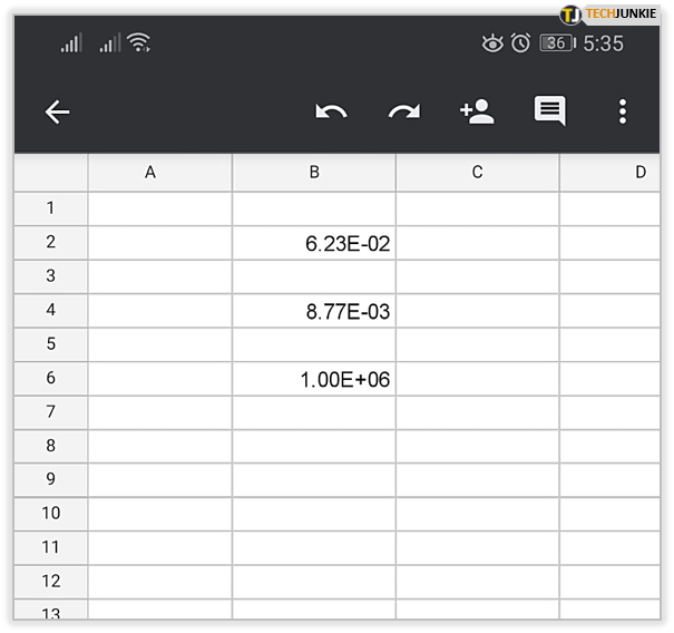
But before we show you the steps, make sure to download Google Sheets. It’s available both for Android and iPhone users. Once downloaded, you can turn off Scientific Notation. Here’s how to do it:

1. Launch Google Sheets.
   
2. Open the spreadsheet where you write numbers.
   
3. Select the cells you need.
   
4. Now, click on ‘Format’ or the ‘A with horizontal lines’ on the top of the screen.
   
5. Hit ‘Cell.’
   
6. Click on ‘Number format.’
   
7. Unselect ‘Scientific’ and click on what you need from the list.
   

Note: Most users should click ‘Number’ because they’ll most likely use it often.

Turning Off Scientific Notation on a Computer

If you usually use Google Sheets on a computer, follow these steps to turn off Scientific Notation:

1. Open Google Sheets and a spreadsheet you use.
   
2. Select a range of cells with numbers.
   
3. Then, go to the menu and click on ‘Format.’
   
4. You’ll see ‘Number’ in the drop-down menu. Hover over it.
   
5. Notice that ‘Scientific Notation’ is turned on.
   
6. To turn off this option, click on any other option.
   

That’s it! You might recognize some of the steps if you already use Excel. Remember, if the ‘Scientific Notation’ turns back on, just follow the steps above again.

Number Formats

You might have noticed various number formatting options when you clicked on ‘Formats.’ These are useful when you’re working with numerical data. It’s much easier to read numbers when you select the right Number Format option. Let’s see which options these are:

Date

When you need to write dates, turn on the ‘Date’ function. Doing so will enable Google Sheets to recognize numerical information as a date instead of a regular text. For instance, if you type ‘December’ in the cell, along with the day and the year, Google Sheets will leave the information as it is. To apply the ‘Date’ function to your cells, here’s what you need to do:

1. Select the cell with the date.
2. Head over to ‘Format’ and then ‘Number.’
3. Click on ‘Date.’
4. Information in the cell will automatically convert into the date.

Note: For Google Sheets to recognize the data, you need to write dates without the ‘th.’ For example, you’ll type in the cell ‘January 25,’ instead of ‘January 25^th.’ If you don’t write the year, Google Sheets will automatically include the current year.

Currency

Do you deal with various currencies in your daily life? If so, the ‘Currency’ function will make your life easier. By enabling this function, the currency symbol shows in front of the number. Moreover, the number is in decima formal. Here are the steps to turning on ‘Currency:’

1. Select the column with the numbers you want to show as currencies.
2. Go to ‘Format’ and hover over ‘Number.’
3. Then, select ‘Currency’ or ‘Currency (rounded)’ to have a rounded number.

Keep in mind that the US dollar will, in most cases, be the default currency. If you work with other currencies, here’s what you need to do to make changes:

1. Select the column with the numbers.
2. Click on ‘Format.’
3. Hover over ‘Number’ and scroll to ‘More Formats.’
4. Here, tap on ‘More currencies.’
5. You’ll see a pop-up window with various currencies.
6. Scroll down until you find the one you need.
7. Then, click on ‘Apply.’

The column will automatically show the new currency.

Time Formatting

Google Sheets has an option to change the way time is formatted. To include the way you see minutes and seconds, here’s what you need to do:

1. Write the time in one cell.
2. Then, click on ‘Format’ and in ‘Number’ go to ‘More Formats.’
3. Here, click on ‘More date and time formats.’

In the pop-up window, you can change the number of leading zeros you would like displayed. Click on ‘Hour,’ ‘Minute,’ or ‘Second’ to do this. Tap on ‘Apply’ when you finish.

Various Number Formatting Options

An average Google Sheets user doesn’t need to have ‘Scientific Notation’ turned on. Luckily, turning it off is easily done if you follow the above steps. Plus, you now know how to use other ‘Number Formatting’ options.

Why do you usually use Google Sheets? Do you have any other cool tips regarding ‘Number Formatting?’ Share with the community in the comments section below.