How To Calculate Standard Error in Excel

Standard error or standard deviation is an extremely handy tool when you want to gain a deeper understanding of the data that’s in front of you. It tells you how much values in a particular data set deviate from the mean value.

There two main varieties – standard deviation for a sample and standard deviation for a population, and they’re both included in Excel. Let’s see how to go about calculating standard deviation in Excel.

Standard Deviation for a Sample

Standard deviation for a sample is one of two major standard deviation functions MS Excel lets you calculate for your charts. It represents the standard deviation from the mean for a selected sample of data.

By using this function, you can easily calculate how much a certain subset of data deviates from the mean value. Let’s say that you have a chart with the salaries of all employees in a company and you only want the data on the salaries in the IT sector. You’ll use the standard deviation for a sample or the STDEV.S function.

Standard Deviation for a Population

Standard deviation for a population is the other major standard deviation function you can calculate through MS Excel. As opposed to the standard deviation for a sample, standard deviation for a population shows the average deviation for all entries in a table. It is marked as STDEV.P in MS Excel.

So, using the same example from the previous section, you would use the STDEV.P function to calculate the deviation for all employees. Excel also lets you calculate other types of standard deviations, though these two are most commonly used.

How to Calculate Standard Deviation with Excel

Calculating standard deviation in Excel is easy and can be done in three different ways. Let’s take a closer look at each of the methods.

Method 1

This is the fastest way to calculate the standard deviation value. You can use it to get both the sample and population deviations. However, you need to know the formulas to make this method work, which is why so many people tend to avoid it.

In this case, we’re working with a three-column chart. Here’s how to do it:

1. Create or open a table in MS Excel.
   
2. Click on the cell where you’d like the standard deviation value to be displayed.
   
3. Next, type “=STDEV.P(C2:C11)” or “=STDEV.S(C4:C7)”. The values in the brackets denote the range of cells for which you want to calculate the standard deviation value. In this example, you want to calculate STDEV.P for cells C2 to C11 and STDEV.S for cells C4 to C7.
   
4. Press Enter.
   
5. If you want to round the result to two decimals, select the results and click on the Home tab.
   
6. Click the arrow next to General to open the dropdown menu.
   
7. Select More Number Formats…
   
8. Choose the Number option.
   

Method 2

The next method is almost as fast as the first one and doesn’t require in-depth Excel knowledge. It is great when you’re in a crunch but don’t want to mess with the formulas. Let’s see how to get the deviations without typing the formulas.

1. Create or open a table in MS Excel.
2. Click on the cell where the deviation result will appear.
3. Next, click the Formulas header in the Main Menu.
4. After that, click the Insert Function button. It is located on the left side.
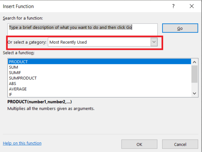
5. Now, click the arrow next to Or select a category to open the dropdown menu.
6. Then, select Statistical, browse the list below and select either STDEV.P or STDEV.S.
   
7. Next, in the Function Arguments window, enter the range for which you want to calculate the standard deviation into the text box next to Number1. Going back to the Method 1 example where we were calculating the standard deviation for cells C2 to C11, you should write C2:C11.
   

When you calculate the standard deviation this way, you won’t need to trim the number, as it will automatically be trimmed to two decimals.

Method 3

There is also a third method, the one that involves the use of Excel’s Data Analysis toolkit. If you don’t have it, here’s how to install it.

1. Start by clicking on File.
2. Next, click on Options, located at the bottom-left corner of the screen of the new window that opens.
3. Now, click the Add-Ins tab on the left side of the window and then click the Go button near the bottom of the window.
   
4. Check the Analysis ToolPak box and then click OK.
   

With the installation complete, let’s see how to use Data Analysis to calculate Standard Deviation.

1. Create or open a table in MS Excel.
2. Click on the Data tab and select Data Analysis.
   
3. Now, select Descriptive Statistics and insert the range of cells you wish to include in the Input Range field.
4. Next, choose between the Columns and Rows radio buttons.
5. Check Labels in First Row if there are column headers
6. Pick where you want the result to appear.
7. Then, check the Summary Statistics box.
8. Finally, click the OK button.
   

You will find the standard deviation for sample in the output summary.

Summary

The standard error or standard deviation value can be calculated in a number of ways. Choose the method that suits you best and follow the steps laid out in this article. Leave any thoughts or comments below.