

How To Compare 2 Columns in Microsoft Excel

There are several different ways to compare data between two columns in Microsoft Excel. Among your options: you can check them manually, you can use a formula or, if the two columns are in different worksheets, you can view them side by side. In this article, I’ll show you a few ways to compare data in Excel.
Also, I’ll wrap this article up by describing a web-based tool you can use for free that enables you to quickly compare to workbooks for differences or duplicates, returning a comma separated values (CSV) showing you the columns you’re comparing side by side according to the comparison criteria you chose.
Compare two columns in Excel
In addition to checking for duplicates between columns of data, you may need to check for differences between columns, especially if one of the columns was changed or the data is from different sources.
In this example, we have a column in Sheet 1 (starting at A1) and another column on Sheet 2 (also starting at A1) that we want to compare. Here’s the process of comparing two Excel columns for differences:
- Highlight the same top cell (i.e., A1) in the column in Sheet1
- Add this formula to the A1 cell: ‘=IF(Sheet1!A1<> Sheet2!A1, “Sheet1:”&Sheet1!A1&” vs Sheet2:”&Sheet2!A1, “”)’
- Drag the formula down the column for each of the cells you want to compare in the two columns in question
The result of this process will be that each duplicate cell will be highlighted in both columns you are comparing. This simple process of checking for duplicates will make you more efficient and productive using Excel.
The differences should then be highlighted as Sheet1 vs Sheet2:Difference1 in the cell containing the differences.
Note that this formula assumes you are comparing Sheet1 against Sheet2 both beginning at cell A1. Change them to reflect the columns you want to compare in your own workbook.
Compare two columns for differences in Excel
So we have checked two columns for duplicates but what if you want to find differences? That is almost as straightforward. For this example, let’s say we have a column on Sheet 1 (starting at A1) and another column on Sheet 2 (also starting at A1) that we want to compare.
- Open a new sheet and highlight the same cell the two columns you’re comparing start on.
- Add ‘=IF(Sheet1!A1<> Sheet2!A1, “Sheet1:”&Sheet1!A1&” vs Sheet2:”&Sheet2!A1, “”)’ into the cell.
- Drag the formula down the page for as many cells as the columns you are comparing contain.
- The differences should then be highlighted as Sheet1 vs Sheet2:Difference1 etc. in the cell where the difference lies.
The formula assumes you are comparing Sheet1 against Sheet2 both beginning at cell A1. Change them to suit your own workbook as you see fit.
Compare two sheets in Excel
If you want to compare data from two different sheets within the same workbook, you can use conditional formatting to do the comparisons, enabling you to compare data using a range of criteria:
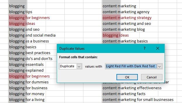
- Open the sheet in which you want Excel to highlight the duplicates
- Then select the first cell in the sheet (e.g., cell A1) then press Ctrl + Shift + End simultaneously
- Click the Home menu, then select Conditional Formatting
- Select New Rule and type ‘=A1<>Sheet2!A1’ into the dialogue box
- Compare A1 Sheet1 against the same cell in Sheet2
- Select a format to display and click OK.
The active sheet should now display the duplicate values in the format you chose. This technique works well if you collate data from multiple sources, providing you a quick way to check for duplicates or differences in the data.
Compare two workbooks in Excel
If you are comparing data from different sources and want to check for differences, similarities or other information quickly by hand, you can do that too. This time you don’t need conditional formatting to do it. Select the View tab then click on the Window group
- Click View Side by Side
- Select View
- Select Arrange All
- ‘Then select Vertical to compare entries side-by-side
The two workbooks will be shown horizontally next to each other by default, which is not ideal for comparing columns. The last step, selecting Vertical displays the columns vertically, making it easier for you to read the results of your comparisons.
If you have longer columns, enable Synchronous Scrolling (from the View Tab in the Windows Group) so that both workbooks scroll alongside each other.
Using conditional formatting in Excel
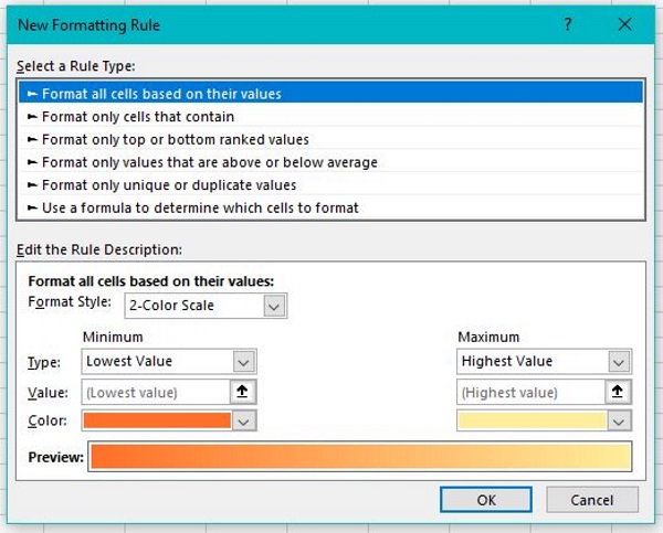
Conditional formatting is an under-used yet very powerful Excel feature that you may find useful. This feature offers some very fast ways to compare and display data in Excel using a set of rules you can use to achieve your conditional formatting objectives:.
- Open the sheet containing the data you want to format
- Highlight the cells containing the data you want to format
- Select the Home menu then click Conditional Formatting
- Select an existing Rule Set or create a new rule set by clicking New Rule
- Enter the comparison parameters (e.g., is greater than 100)
- Set a format to display the results and select OK
Excel will then highlight the cells meeting the criteria you selected (e.g., greater than 100). You’ll find this method a valuable addition to your Excel toolset.
There are some comparison tools for Excel that make comparisons fast and efficient. For example, the Xlcomparator (do a quick web search to find it) allows you to upload the two workbooks you want to compare then go through a step-by-step wizard that guides you through the process, returning a single Comma Separated Value (CSV) file that you can open in Excel to view the compared columns side-by-side.
Do you have any Excel comparison tips or tricks? Please let us know below!