How to Remove Subtotals from Excel

Microsoft Excel allows you to work wonders with your spreadsheets. This is especially true when working with multi-year financial calculations. In order to organize that mess of rows, columns, and thousands of cells, you can use Excel’s “Outline” options. This allows you to create logical groups of data, along with relevant subtotals and totals.

Of course, at some point it may turn out that the overwhelming number of those subtotal rows trashes your financial analysis. But removing them manually is both tiresome and can interfere with the spreadsheet’s integrity. Worry not though, Excel has a solution for that as well.

Removing Subtotals from Standard Spreadsheets

Whether you simply want to remove subtotal rows from your spreadsheet or reorganize the entire sheet, the process is basically the same. Follow the steps below to do so:

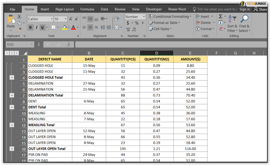
1. Open the Excel spreadsheet you want to edit.
   
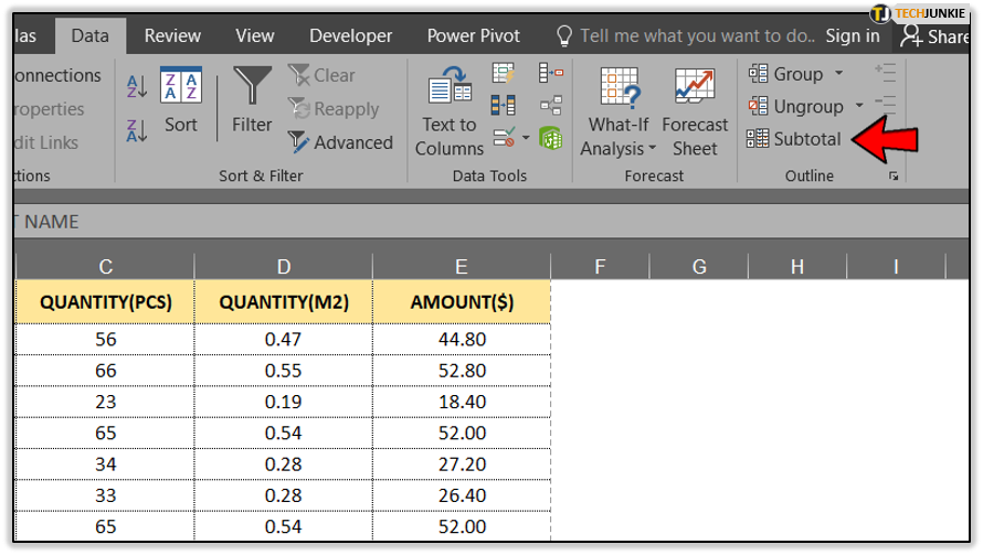
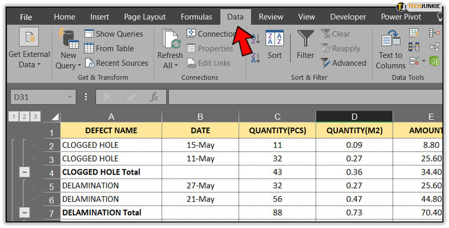
2. Click the “Data” tab.
   
3. In the “Outline” section of the top menu, click “Subtotal”.
   
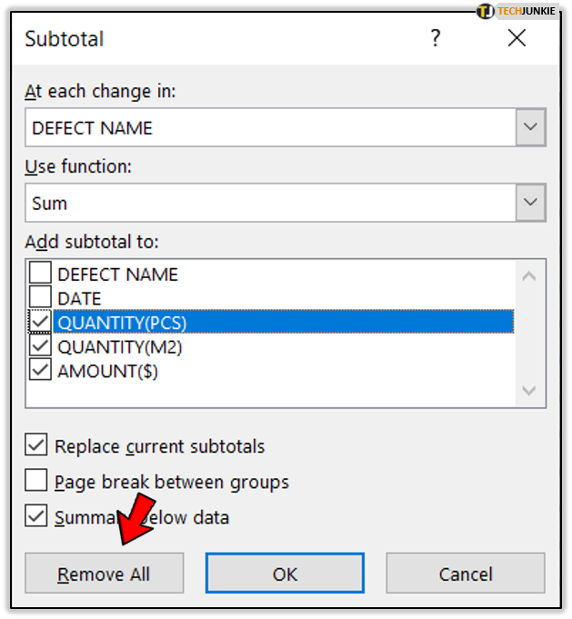
4. In the “Subtotal” menu, click the “Remove All” button.
   
5. This will ungroup all the data in the spreadsheet, effectively removing any subtotal rows you might have there.
   

If you don’t want to delete the subtotals, but want to remove all groups to further rearrange your data, do the following:

1. Click the “Data” tab.
   
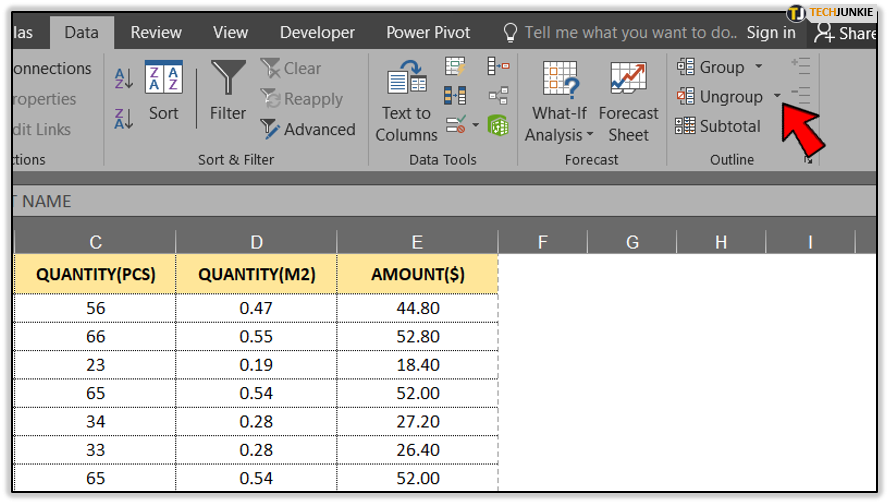
2. In the “Outline” section, click the “Ungroup” drop-down menu.
   
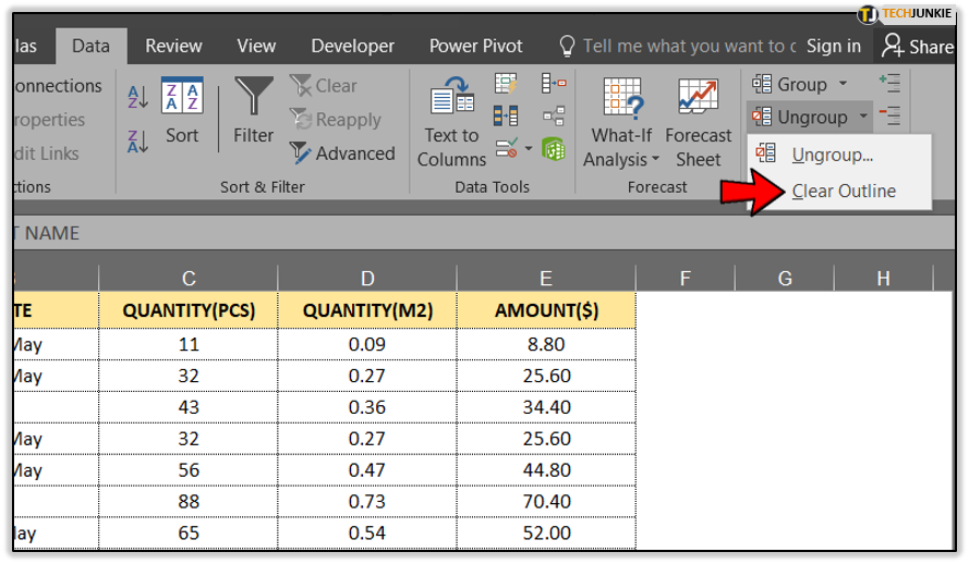
3. Now click the “Clear Outline” option to remove any grouping for that spreadsheet.
   

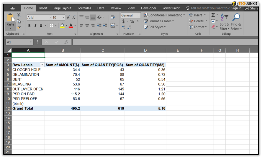
Removing Subtotals from Pivot Tables

If you’re working with pivot tables in Excel, there’s no need to create a new table only to remove the subtotals. You can do that without deleting the entire pivot table.

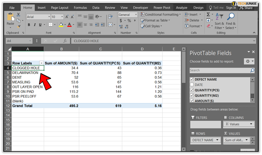
1. Open the Excel file containing your pivot table.
   
2. Now select a cell in any of the table’s rows or columns.
   
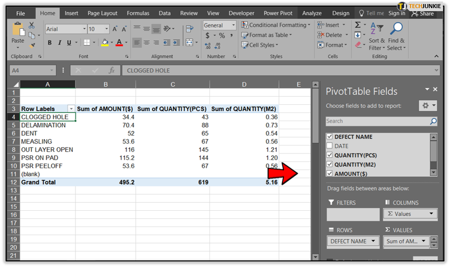
3. This will allow you to access the “PivotTable Tools” menu. It will appear in the top menu, right next to the “View” tab, and will contain two tabs: “Analyze” and “Design”. In older versions of Excel (Excel 2013 and earlier), you’ll see the “Options” and “Design” tabs without the “PivotTable Tools” title above them.
   
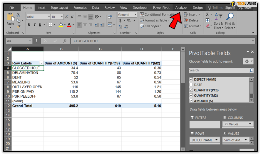
4. Click the “Analyze” tab. For older versions of Excel, click the “Options” tab.
   
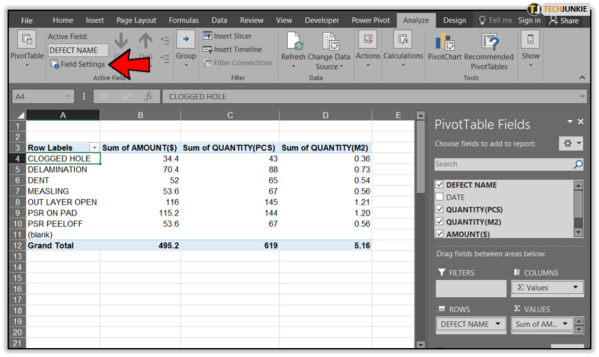
5. In the “Active Field” section, click “Field Settings”.
   
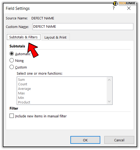
6. In the “Field Settings” menu, click the “Subtotals & Filters” tab.
   
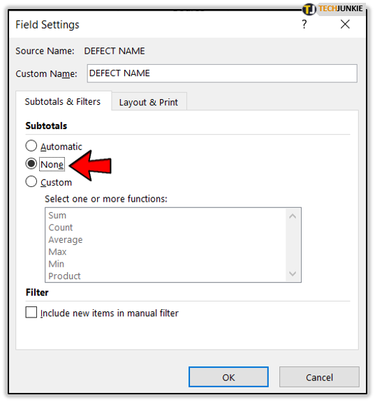
7. In the “Subtotals” section, select “None”.
   
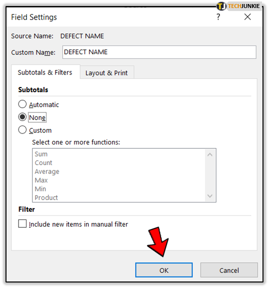
8. Now click “OK” to confirm the changes.
   

Please note that if there’s a field in your pivot table that contains some calculations, you won’t be able to remove the subtotals.

Adding the Subtotals to Your Spreadsheet

Hopefully, you’ve managed to remove the subtotals using the guidelines from the previous two sections. When you’re done rearranging the data in your spreadsheet, you might want to add a new set of subtotals. To do so, please follow the steps below:

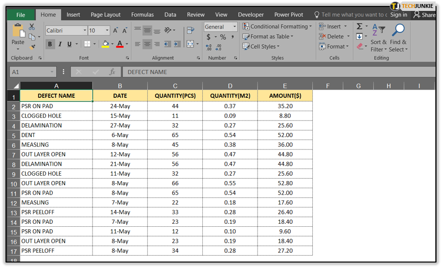
1. Open the spreadsheet in which you want to add subtotals.
   
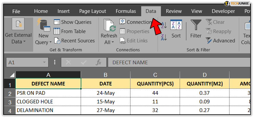
2. Now click the “Data” tab from the top menu.
   
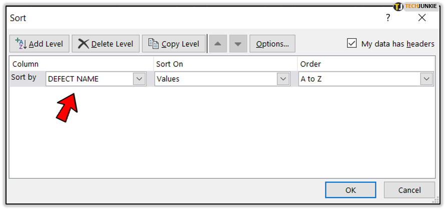
3. Select Sort from the menu and sort the entire sheet by the column which contains the data you want to have subtotals of.
   
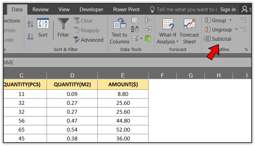
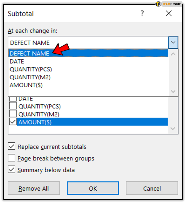
4. In the “Outline” section, click “Subtotal” to open the corresponding menu.
   
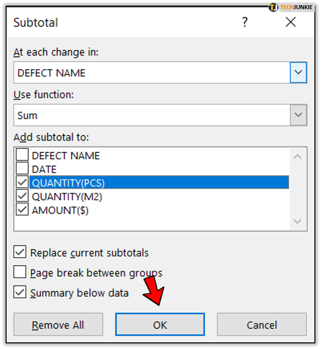
5. In the drop-down menu for “At each change in”, select the column that contains data you want to use for the subtotals.
   
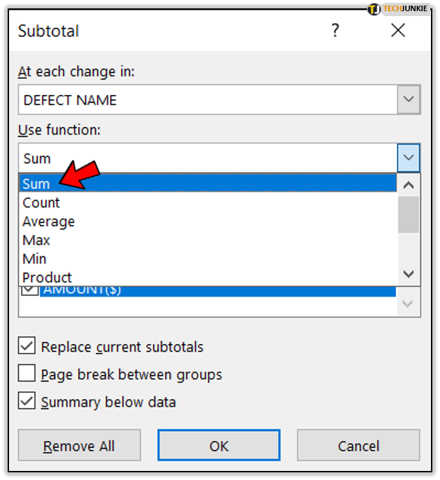
6. Next, you have to choose which operation the subtotals should calculate. In the “Use function” drop-down menu, choose one of the available options. Some of the most common operations are Sum, Count, and Average.
   
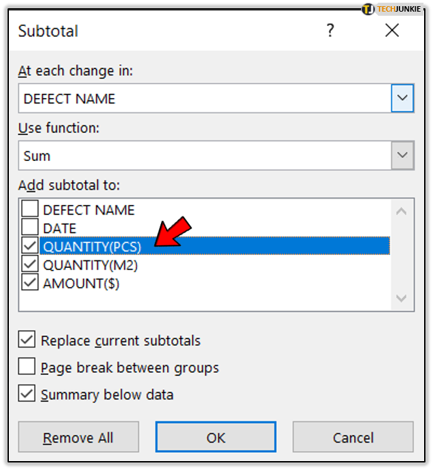
7. In the field “Add subtotals to”, select the column in which you want the subtotals to appear. Usually it’s the same column for which you’re doing the subtotals, as defined in Step 5.
   
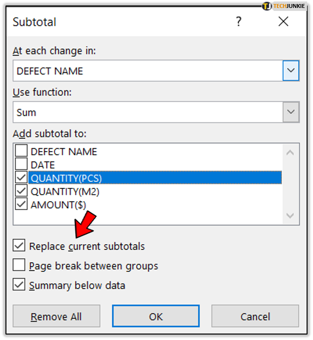
8. You can leave the “Replace current subtotals” and “Summary below data” options checked.
   
9. Once you’re satisfied with your selection, click “OK” to confirm the changes.
   

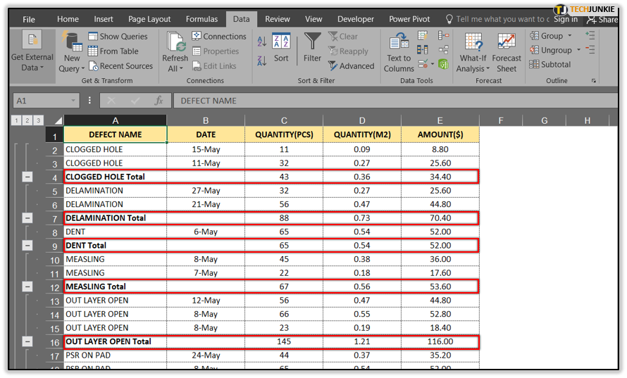
After you click OK, you should see that the rows in your spreadsheet are now arranged into groups. Below each group, a new row will appear, containing the subtotal for that group.

Using Levels to Organize Your Data

When you add subtotals, you’ll notice a new column between the row numbers and the left edge of the Excel window. At the top of this column, there are numbers one, two, and three. These represent the grouping levels for your data.

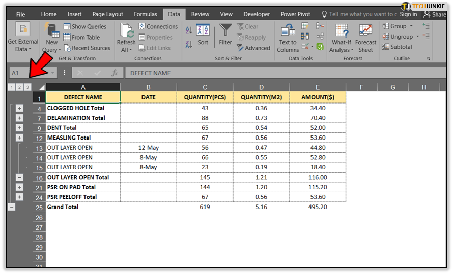
When you click the number three, you’ll be able to see your entire dataset, showing each row, the subtotal rows, and the grand total row. If you click on number two, data will now collapse to show you only the subtotal and grand total rows. Click on number one, and you’ll see only the grand total row.

When you expand everything by clicking the number three, you’ll have “-“ and “+” signs on the levels column. Use these to manually collapse and expand each group on its own.

Thanks to this feature, Excel allows you to hide from view certain portions of your spreadsheet. This is useful when there’s some data which isn’t essential to your work at that moment. Of course, you can always recall it by clicking the “+” sign.

Subtotals Removed!

Thanks to Excel’s powerful tools you now know how to avoid a lot of unnecessary manual work when removing subtotals. After you rearrange all of the data, it’s only a simple matter of clicking a few Excel options to add those subtotals back. Also, don’t forget to use levels to optimize the way you view your data.

Have you managed to remove subtotal rows from your spreadsheets? Do you find this a better option than manual removal? Please share your thoughts in the comments section below.