How to Multiply Column by Constants in Google Sheets

Google Sheets is an incredibly useful program that allows you to input relevant data, and make various calculations. The formulas can help you make estimates, manage a budget, and calculate taxes.

Google Sheets is mainly designed for creating lists. So when you apply a formula, the program will show different numbers as you move down the list. Often, you’ll need to multiply a column by the same number. The steps are simple. Just go through this guide and you’ll be able to do it in no time.

Multiplying Columns by the Same Number

If you want to multiply cells or columns by the same number, you’ll have to use an absolute reference. This will help you have a constant in the formula across cells.

The absolute reference is represented by a dollar sign ($). To multiply columns by the same number, you need to add $ to numbers in a formula.

To apply any formula in Google Sheets, you have to know which signs you should use. Let’s take a look at them:

1. All formulas must begin with an equality sign (=).
2. You should write an equality sign in the cell where you want your formula and numbers to show.
3. To multiply numbers in cells, use an asterisk (*).
4. Finally, press ‘Enter’ to calculate and complete your formula.

Now that you know these basic points about Google Sheets formulas, let’s see how to apply them to multiply cells by constant.

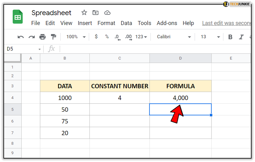
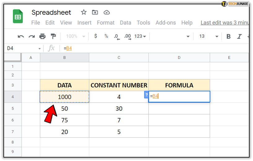
Take a look at Google Sheets below.

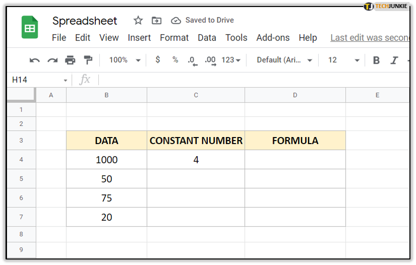
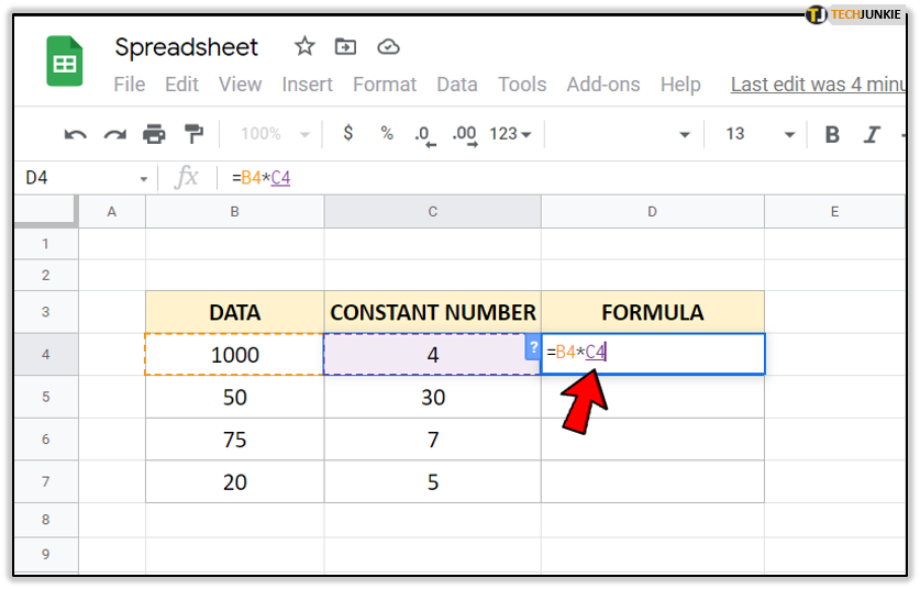
In this example, you can see we have some numbers in the B column, which we want to multiply by a number in the C column. To do so, follow these steps:

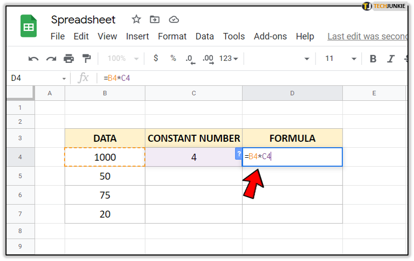
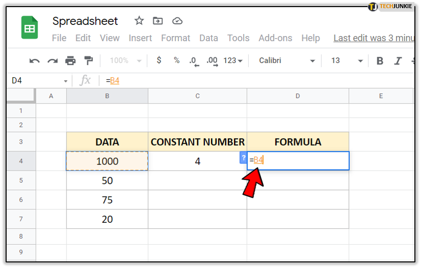
1. Make sure your cursor is in a cell D4.
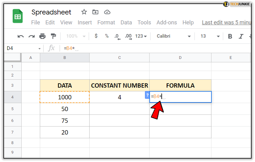
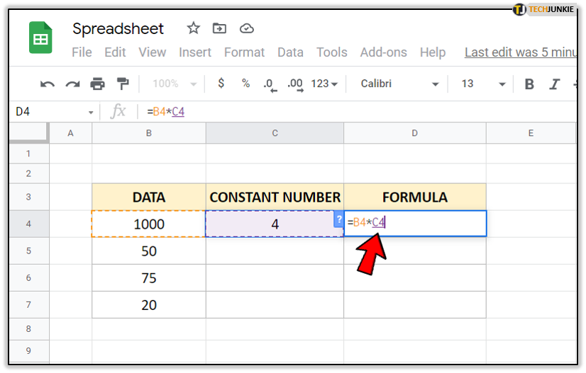
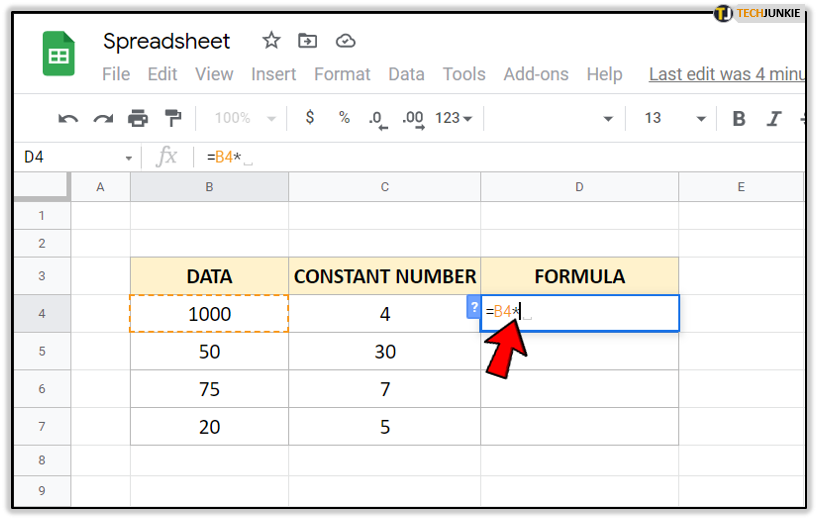
2. Type the following: =B4*C4.
   
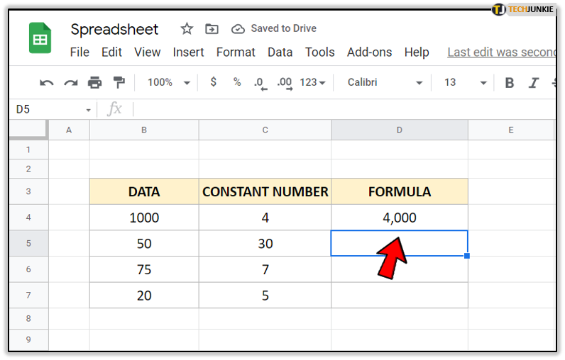
3. This formula will multiply the two cells and give you the correct result.
   

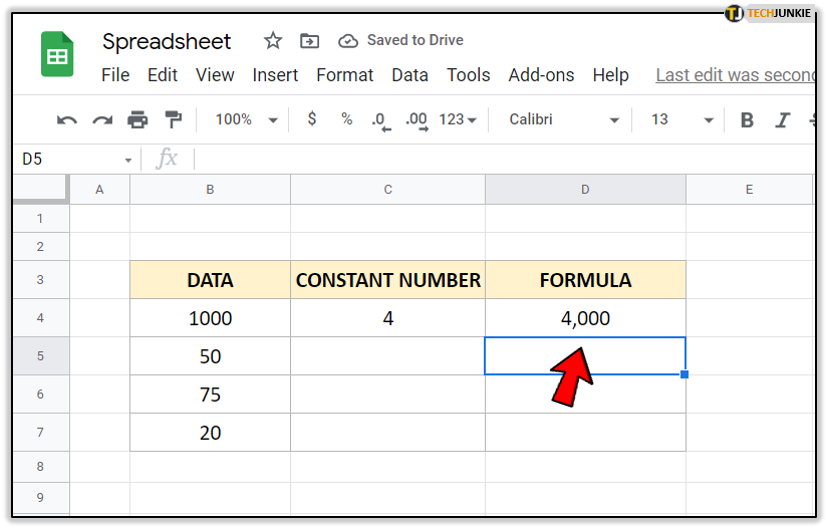
However, if you want to copy down that formula, it unfortunately won’t work. You’ll just get zero in the other D cells.

So to multiply every number in column B by a number in C4, you’ll have to add an absolute reference as we’ve mentioned. Here’s how to do it:

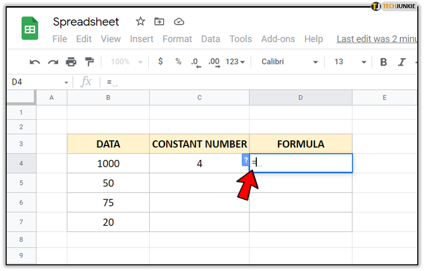
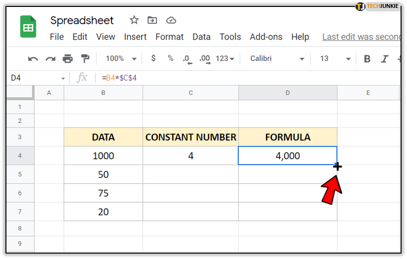
1. First, in D4 write an equality sign (=).
   
2. Next, either click on B4 to add it to the formula, or type it after ‘=.’
   
3. Now type an asterisk sign (*).
   
4. Click on C4 to enter the formula in the cell, or simply type it.
   
5. Then, insert ‘$’ in front of C and in front of the number of the cell. It should look like this ‘$C$4.’
   
6. Press ‘Enter’ to get the formula.
   

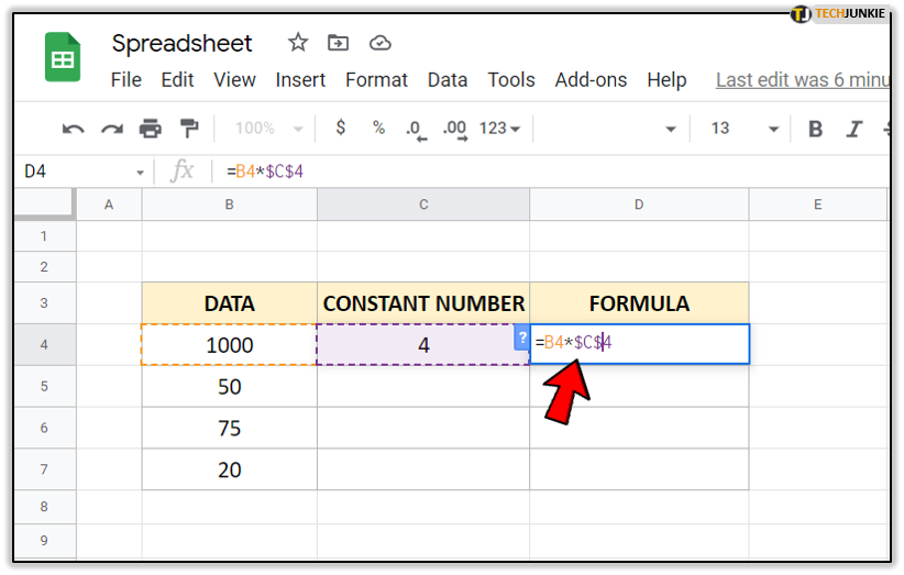
By putting ‘$’ in front of the letter and number of the cell, you suggest that C4 is ‘absolute’. This means that when you copy the formula to another cell, it will always take C4 as the reference number.

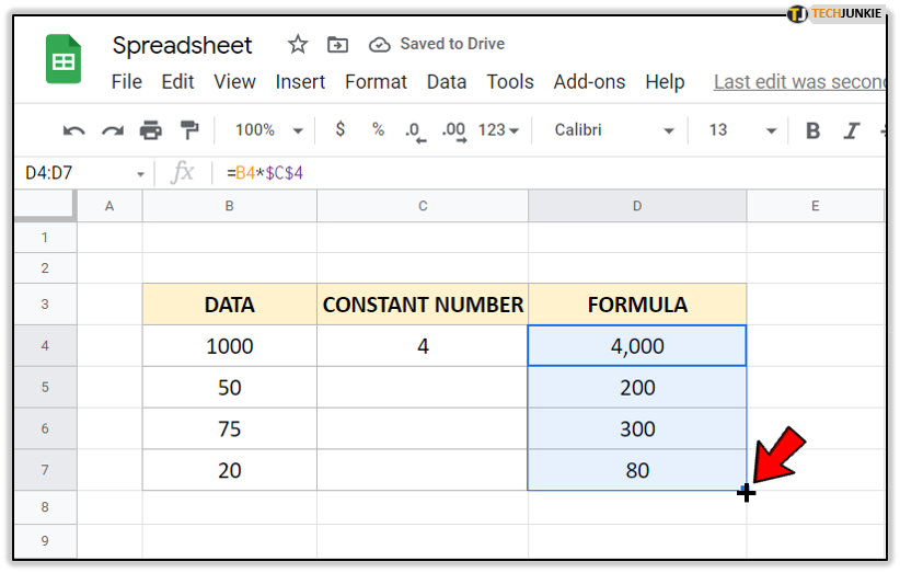
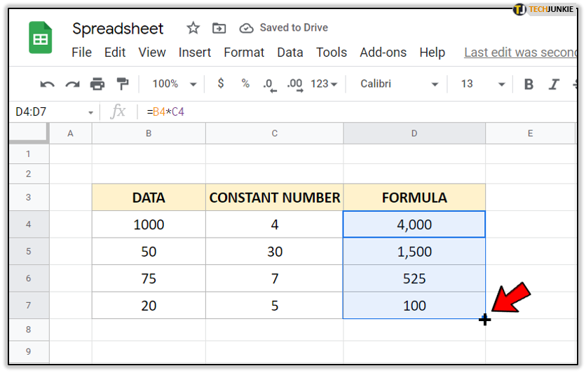
Now, if you want to copy this formula down the column, follow these steps:

1. Select D4.
2. Next, Point the cursor on the square in the bottom right corner of the cell. You will notice that the pointer will be turned into crosshair symbol ‘+’.
   
3. Drag down the formula.
4. It’ll copy down the D column.
   

Note: You can double-click on all cells to check if the formulas are correct. The basic formula should be the same in all of them, including the absolute reference. Other details, like the cell number, should differ.

Multiplying Two Columns

Multiplying two columns is quite easy. However, if you have to multiply many cells in each column, you don’t want to do it manually as it isn’t time-efficient.

Here’s how to multiply numbers from two columns quickly:

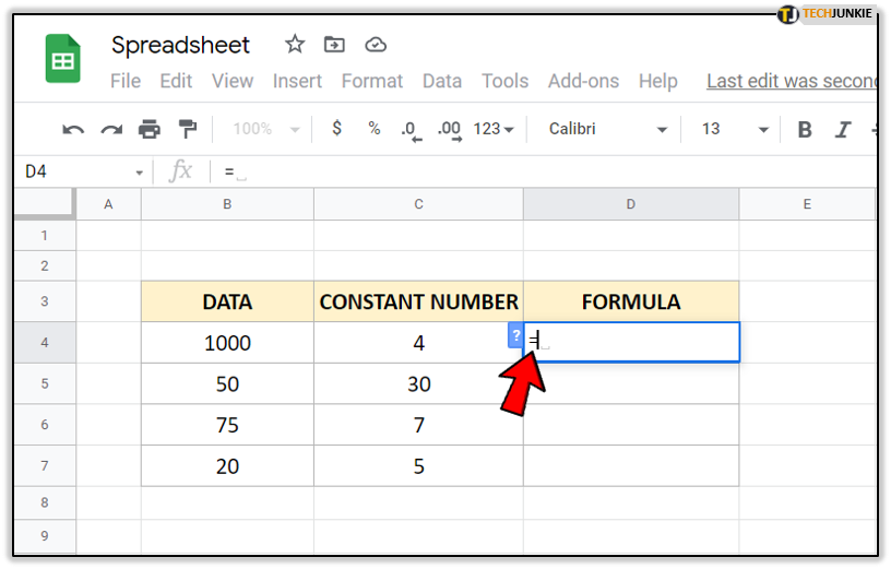
1. Select the column where you want the product to appear. In our example, it’s D4.
2. Next, add an equality sign (=).
   
3. Click on the first cell you need multiplied. Here, it’s B4.
   
4. Add an asterisk sign (*).
   
5. Then, click on the cell which you want to multiply. In our example, it’s C4.
   
6. Tap ‘Enter’ to get the product.
   

To get multiplications for all cells, simply click on the small square in the bottom right corner of the formula and drag it down.

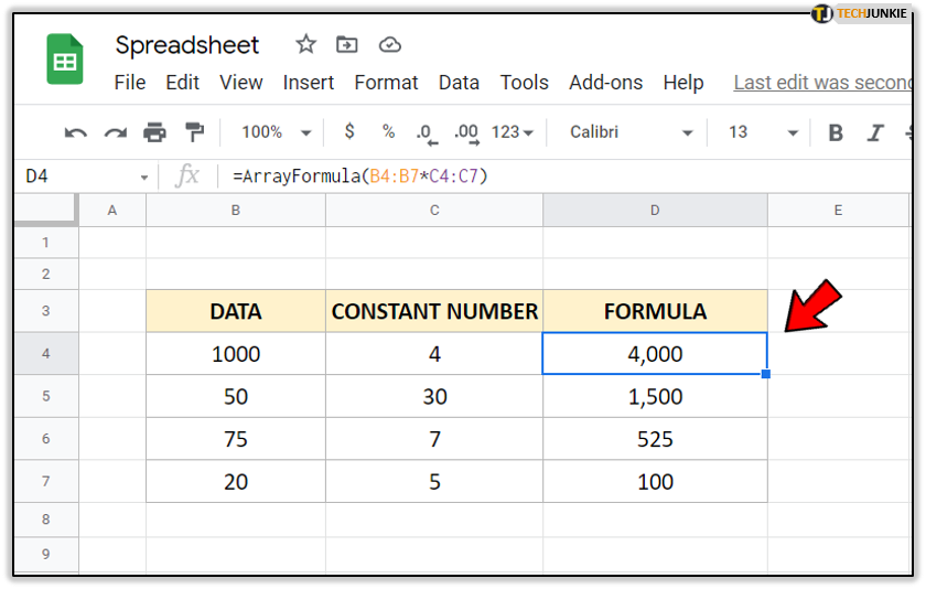
Multiplying Columns Using an Array Formula

Using array formulas is an efficient way to do multiple calculations. Let’s say you have two columns with data, you want to multiply them, and then get the total cost. You could do this manually, but you’ll lose time. Instead, you should use an Array Formula.

For instance, you want to have the sum in the separate cell. If you apply the regular formula of multiplying the cells, you’ll get an error.

To fix this, do the following:

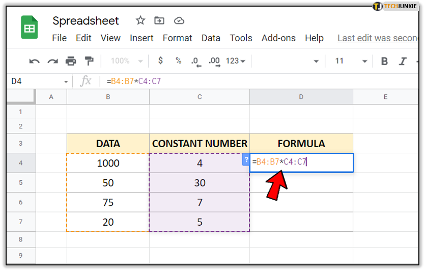
1. Click on the cell where you want formula to show.
2. Type the same formula you’d use for multiplying. Here, it’ll be ‘=B4:B7*C4:C7.’
   
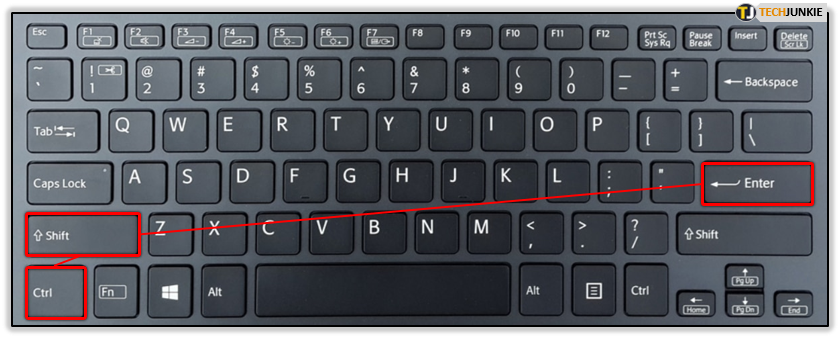
3. Now, hold Ctrl + Shift + Enter, or Cmd + Shift + Enter for Mac users.
   
4. Google Sheets will automatically add an array formula.
   

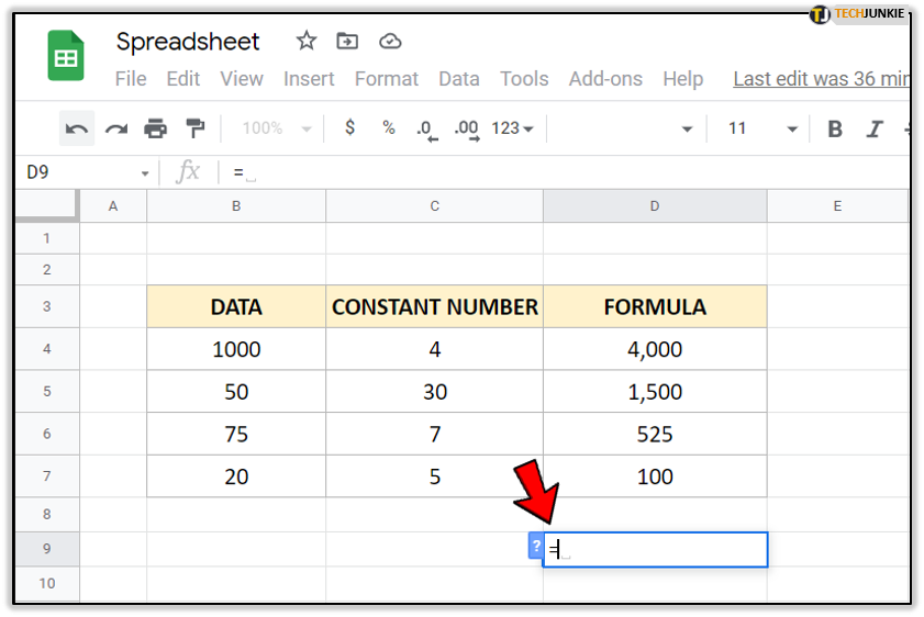
Now, since you need to add a sum, you’ll have to apply another formula.

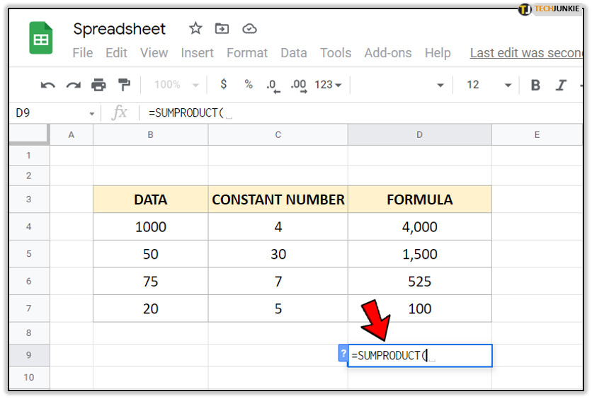
1. Select the cell where you want to add the product of data.
2. Type an equality sign (=).
   
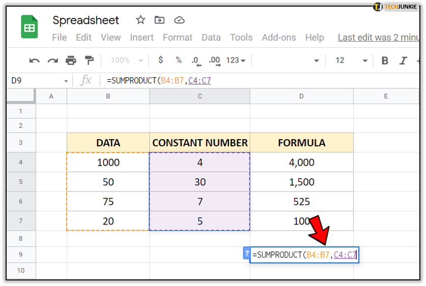
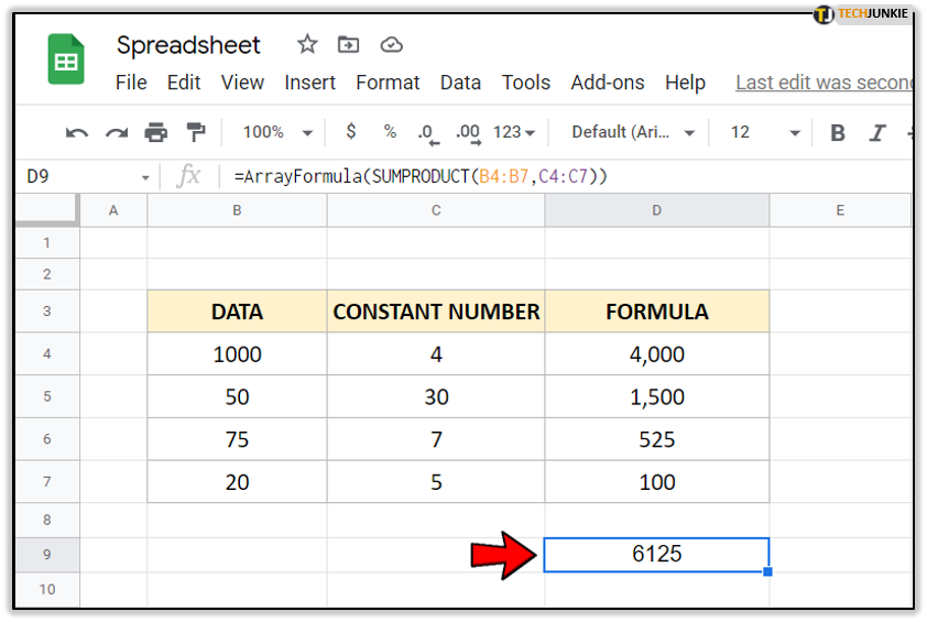
3. Then, write down ‘SUMPRODUCT(’ next to it.
   
4. Select the range of cells you want to multiply.
   
5. Hold down Ctrl + Shift + Enter, or Cmd + Shift + Enter for Mac users.
   
6. Tap ‘Enter’ to get the sum of the product.
   

Google Sheets Multiply Functions

In the past, you might have had issues with the multiplying function. Not anymore. Now you know how to multiply columns by constant, use an Array Formula, and multiply two columns.

Have you ever used any of the methods from this guide? Do you have other tips for our readers? Feel free to share them in the comments section below.