

How To Hide Columns In Google Sheets
Google’s GSuite is one of the most popular platforms on the internet. For both professionals and personal users, the combination of Google Sheets, Google Drive, Google Docs, and other software work to provide a powerful collection of products that any user would be happy to work with.
That said, with all of these different offerings, there are tons of different ways people can take advantage of the software. Some of these uses are easy to figure out, such as organization tactics within the pieces of software. Others are somewhat complex, such as editing legends within sheets or organizing different charts.
If you want to be recognized for your proficiency within this software, it’s vital that you learn the different ways to utilize it. If you do so, you’ll be able to market yourself professionally to others and get paid for your expertise within the GSuite.
To help you on your journey, we’re going to show you a useful feature within Google Sheets. That’s right, this guide is focusing on how to hide columns within Google Sheets.
How To Hide Columns In Google Sheets
As you may know, Google Sheets is the GSuite’s version of Excel. This edition comes with cloud storage and different ways to collaborate with users that have access to the platform. Collaborators can work on the same sheet together at the same time, with the platform storing the history of edits for everyone to look back on whenever they’d prefer.
However, sometimes when you’re working, there may be columns within Google Sheets that you don’t need to look at. A clean workspace is a comfortable workspace, is it not?
Regardless of if you’ve put information into the different sheets and columns available to you, you can hide them from view to make your work experience a little easier for yourself. Not only that, but you can hide rows as well to customize the workspace even more.
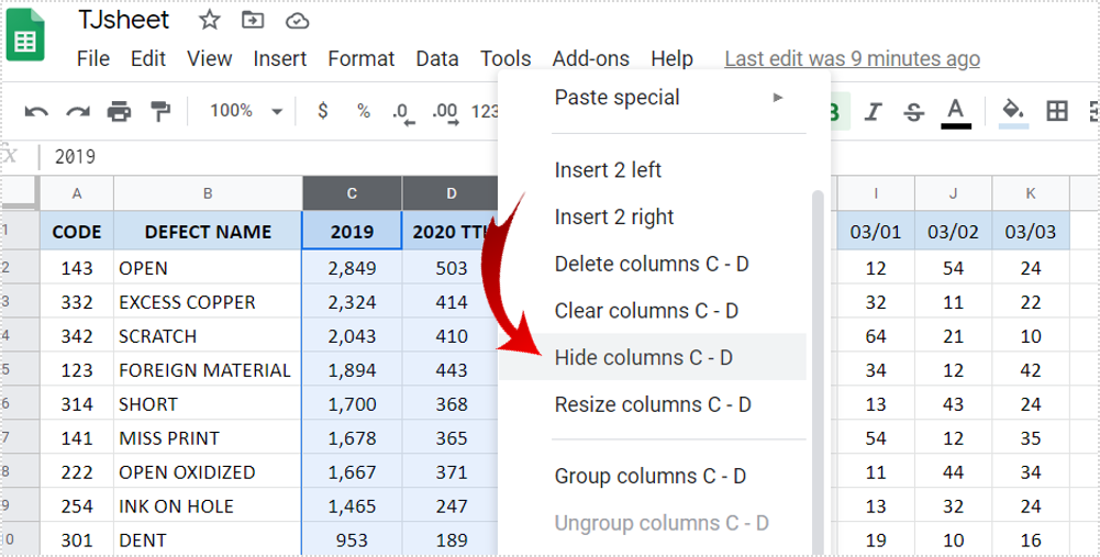
If you want to hide a row or a column within Google Sheets, simply follow these steps:
- Log into your preferred Google Sheets spreadsheet by heading to the Google Sheets website and accessing it with your Google account.

- Use your left mouse click-and-drag to select an array of rows and columns.

- Once selected, right click on the grouping and select “hide row” or “hide column.”

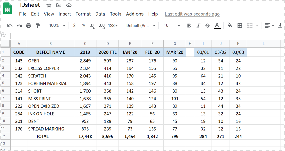
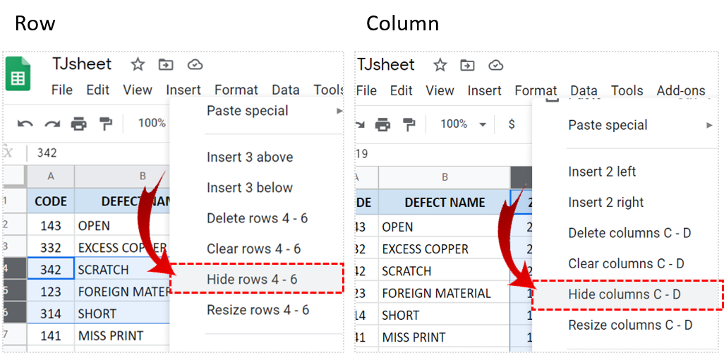
There you have it! Now your columns and rows are hidden. However, if you ever want to reenable the hidden items, we can show you how to do that too.
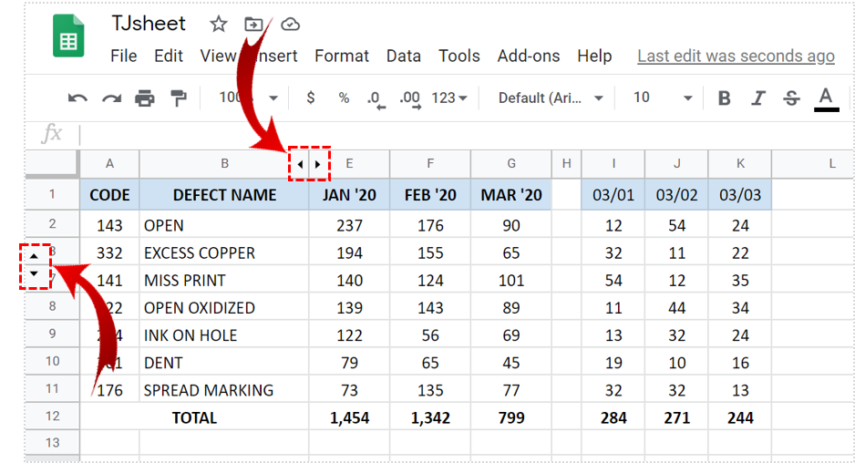
Within Google Sheets, any of your hidden columns and rows will be represented by arrows that link between the start and end of the hidden items. For example, if you chose to hide columns C and D, the two arrows would appear between B and E. Simple click this arrow to make the hidden items appear again.
Now that you know how to hide columns and rows in Google Sheets, you should know that you can also manipulate rows and columns to your will. We’re going to show you how as a little bonus.
How To Manipulate Rows and Columns in Google Sheets
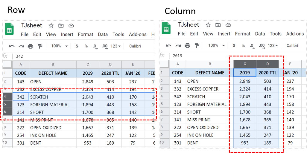
Within the Google Sheets spreadsheet, make sure you select the rows and columns you’d like to manipulate. You can do so by taking your left-mouse button, clicking it down, and holding it while dragging it across the desired cells.
From here, you’re going to select the Edit tab on the top left of the spreadsheet. Then, there are an array of different options for you to pick that allow you to manipulate the selected rows and columns.
Per the selected options, here are a few highlights:
Moving A Row Or Column
Depending on if you’ve picked a row or a column, you can move the information up/down and left/right, respectively. Simply select the rows or columns, go to the Edit tab and choose the move option within the list.
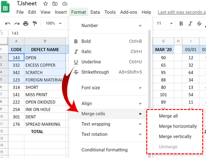
Merging Cells
You can also merge cells within Google Sheets. To do so, simply select an array of cells you’d like to merge, head up to the “Format” tab on the top left of the screen, maneuver to “Merge cells,” and select between “Merge all,” “Merge horizontally,” or “Merge vertically.” You can also do the same with rows and columns by following similar steps.
Change Row Height
As more of a quality of life touch, you can also manipulate the row height within a Google Sheets spreadsheet. This can be done manually or by entering in different inputs.
To do so manually, simply hover your mouse under or on top of the row you want to edit. Click and drag either up or down and adjust to your heart’s content. Otherwise, if you’re going to do entering in different inputs, just right-click on the number of the row you want to modify. From here, go down the drop-down list into “Resize Row.” A pop-up box will appear, and you can enter in your desired row height in pixels. Click okay once done, and you’re set!
Hopefully you enjoyed this guide on Google Sheets and its hiding and adjustment features. Don’t forget to check out our other software guides all over TechJunkie!