How to use VLOOKUP in Excel

VLOOKUP is the go-to tool for finding information in large or complicated spreadsheets. Essentially it’s a search function and along with HLOOKUP, can seek out values across the entire sheet. It is an amazingly useful tool that anyone who spends any time in Excel needs to know. Here’s how to use VLOOKUP in Excel 2016.

VLOOKUP is more than just using Ctrl + F in other Office documents. It is a full vertical (hence the ‘V’) lookup tool that can search the first column of a sheet for anything contained within it. Along with HLOOKUP (the Horizontal lookup tool), they allow you to search quickly and efficiently.

VLOOKUP in Excel 2016

To make VLOOKUP work in Excel 2016 you need three pieces of information, the value you’re searching for, the data to search and the results column to place those results. They are expressed as lookup_value, table_array, col_index_num and range_lookup or:

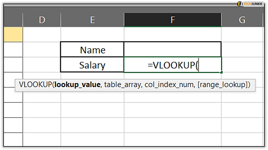
VLOOKUP(lookup_value,table_array,col_index_num,[range_lookup])

• lookup_value is what you’re looking for.
• table_array is the cell range to search.
• col_index_num is data to search for.
• range_lookup is whether you want an exact or approximate match.

How to use VLOOKUP in Excel

So now you know what VLOOKUP is, how do you use it? Let us build your formula up step by step making it easy to understand.

You may notice ‘$’ between characters within the formula, these tell Excel the terms are absolute and to not mess with them. It makes life a lot easier even if it does make the formula harder to read.

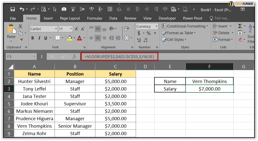
The formula we are going to end up with is ‘=VLOOKUP($F$2,$A$2:$C$55,3,FALSE)’

Here’s how to build it.

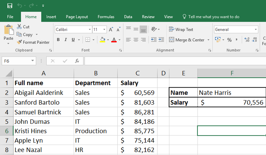
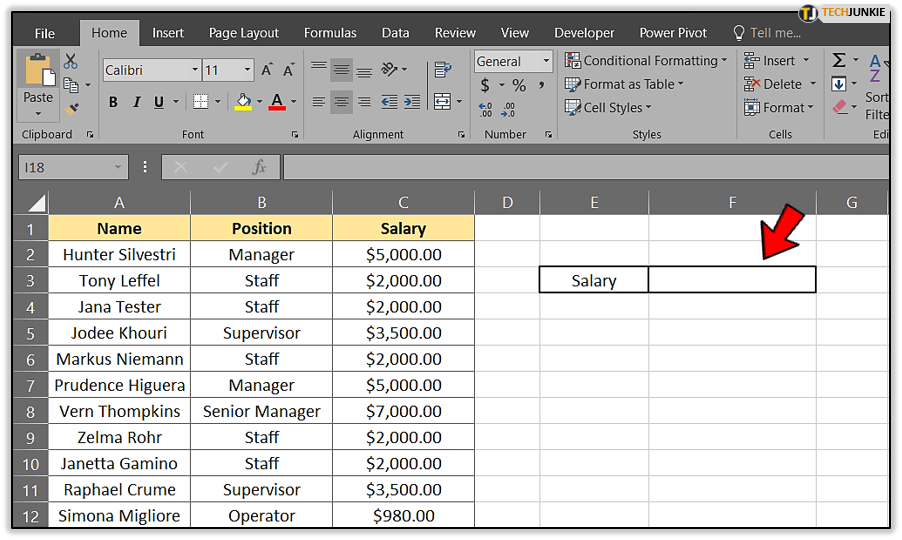
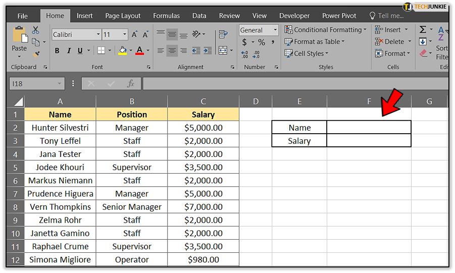
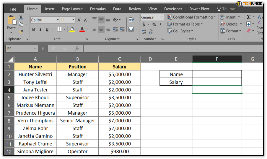
1. Open your spreadsheet and find somewhere to place the results. Put a box around it or otherwise mark it out so you can see clearly what is returned. (Cell F3 in our example).
   
2. Add a box above it in which to put your search criteria. (Cell F2 in the example).
   
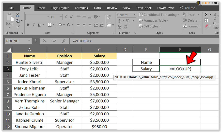
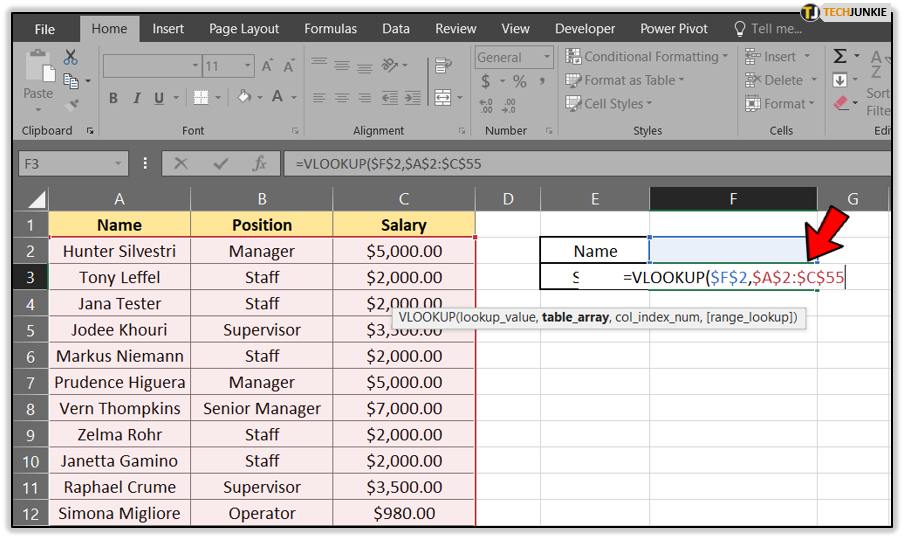
3. Type ‘=VLOOKUP(‘ into F3 where you would like your data displayed.
   
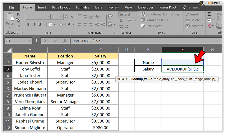
4. Add where you want the data displayed. For example, if you’re sending the result to F2, your lookup should look like: ‘=VLOOKUP($F$2’.
   
5. Add the search area of the spreadsheet. In the example, that’s cells A2 to C55. ‘=VLOOKUP($F$2,$A$2:$C$55’.
   
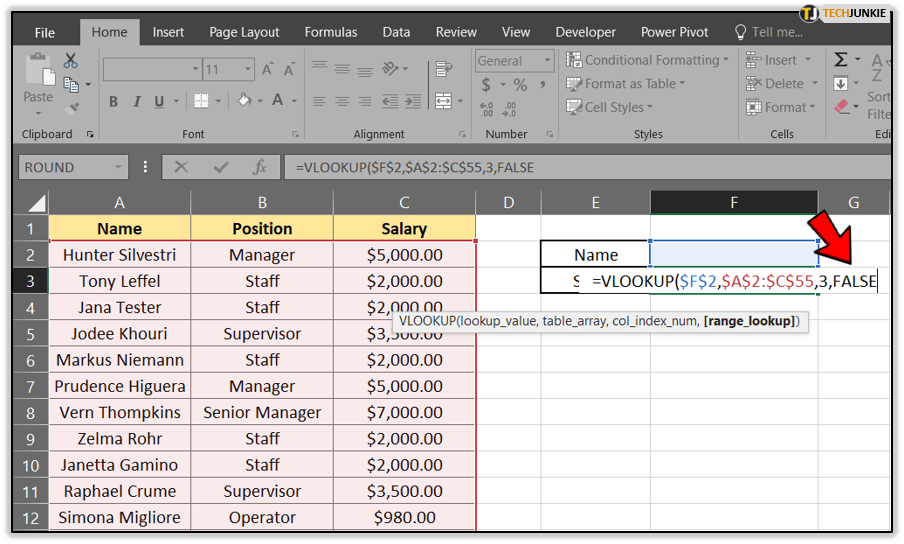
6. Tell Excel what value you’re looking for. In the example, that is salary so we use column 3. ‘=VLOOKUP($F$2,$A$2:$C$55,3’.
   
7. Tell the spreadsheet whether you need an exact match or approximate by adding TRUE or FALSE. We want an exact match so: ‘=VLOOKUP($F$2,$A$2:$C$55,3,FALSE’.
   
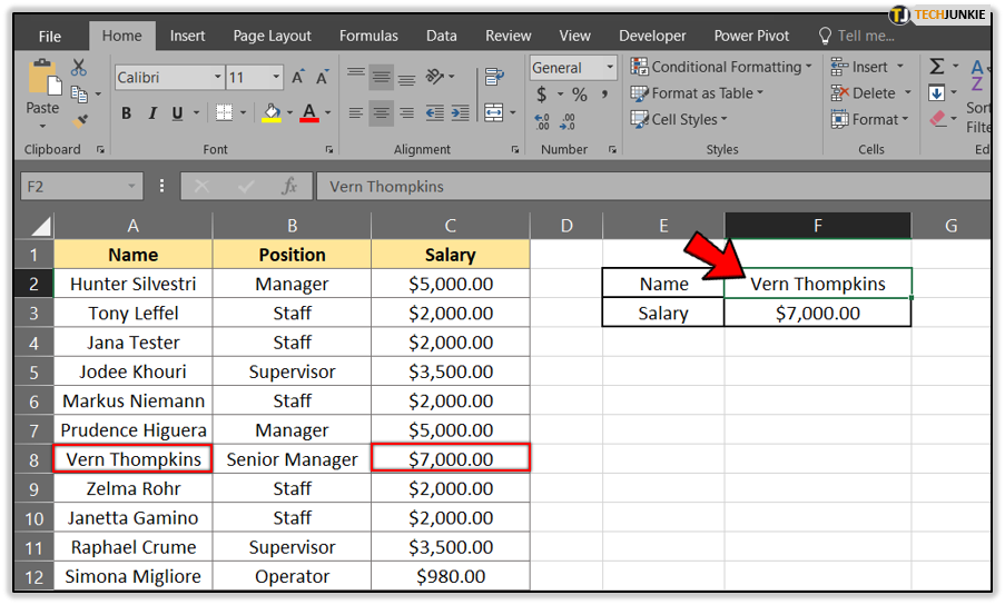
8. Hit Enter.
   
9. Type a search criteria into the box at F2 you created in step 2 and see the return in the box below at F3.
   

There you have it, the anatomy of VLOOKUP in Excel 2016. It is a powerful tool that makes life much easier when dealing with larger spreadsheets.

Thanks to Spreadsheeto.com for the sample.