How to Make a Row Sticky in Google Sheets

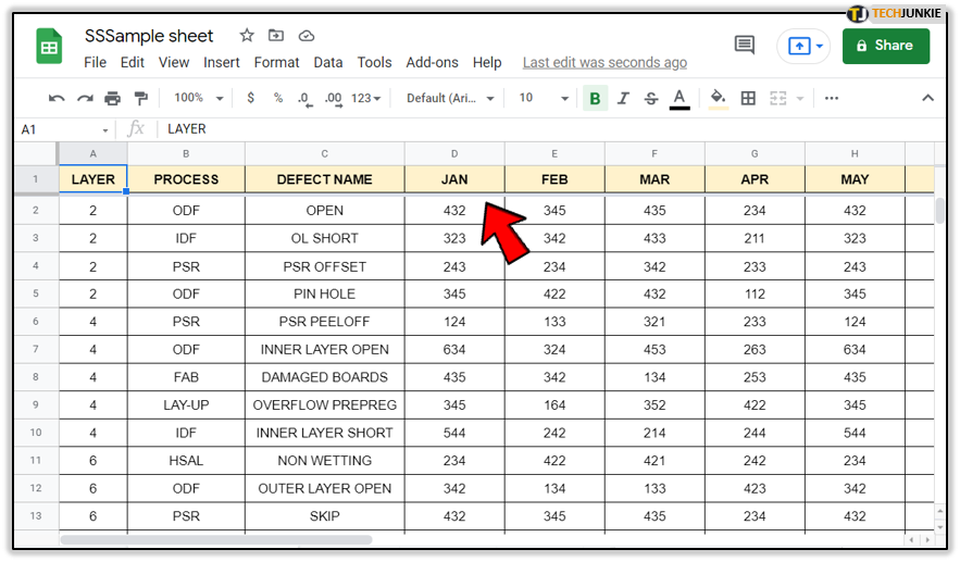
If you’ve ever used a worksheet with a lot of entries, you’ll notice that when you scroll down, everything scrolls down with you. This is a hassle if you want to keep seeing the header rows of a particular worksheet. Fortunately, there are ways to enable that.

In this article, we’ll show you how to make a row sticky in Google Sheets, along with some other useful tips.

Freezing Rows or Columns

The actual command to make a row or column sticky is to Freeze them. Using Freeze will lock the rows or columns that you designate in place. This command is available on PC, Android, and iOS by doing the following:

On PC

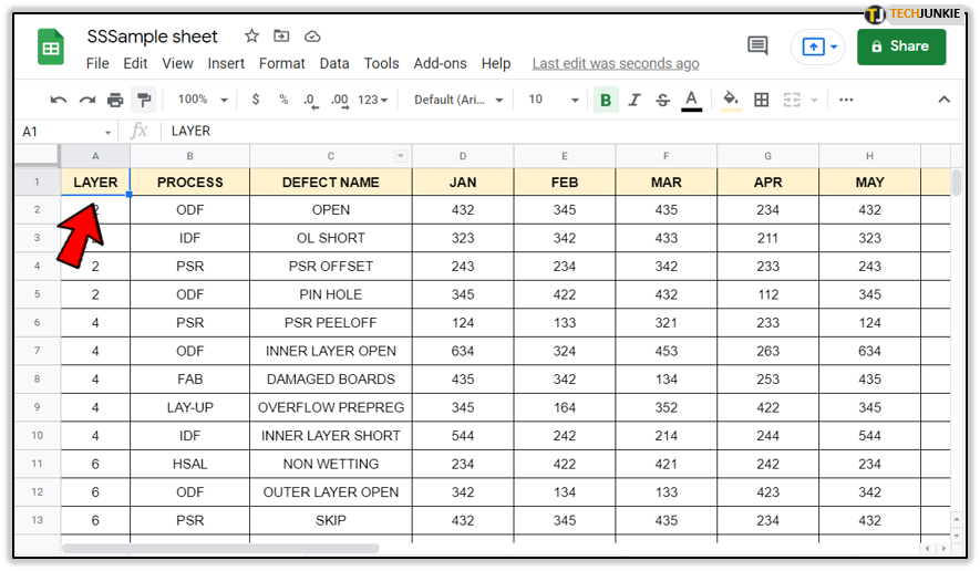
1. Select the rows or columns that you want to Freeze.
   
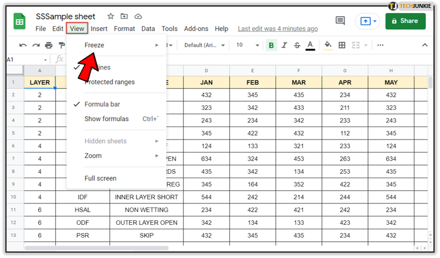
2. On the top menu, click on View, then hover over Freeze.
   
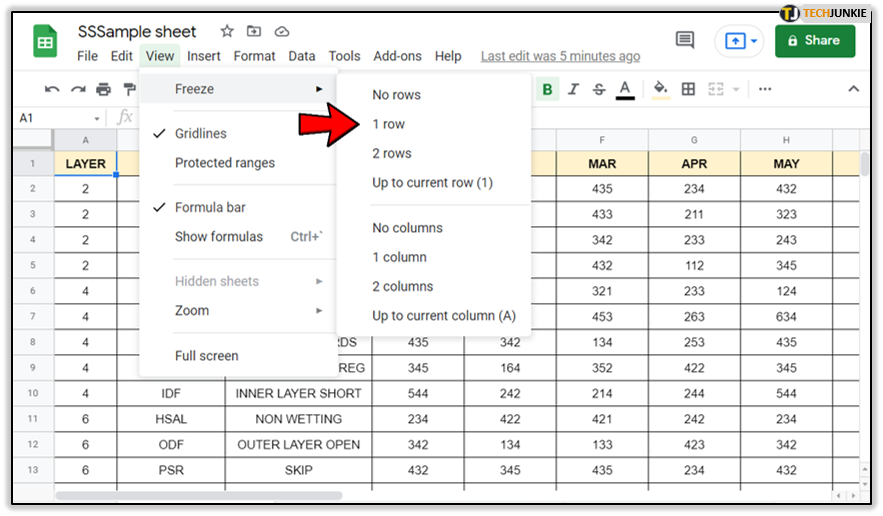
3. Select the number of rows that you wish the command to apply to. Choosing No Rows will unfreeze any row or column currently frozen. Choosing one or two rows or columns will freeze that many rows or columns. The option to Freeze up to current will allow you to freeze all rows or columns up to your current selection.
   
4. The frozen row will be indicated by a gray line running horizontally or vertically through the sheet. You can move a currently defined Freeze selection by clicking and dragging that line to your desired placement.
   

On Android

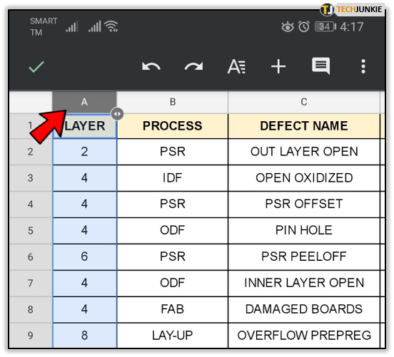
1. Select the row or column that you wish to freeze by pressing on its row number or column header.
   
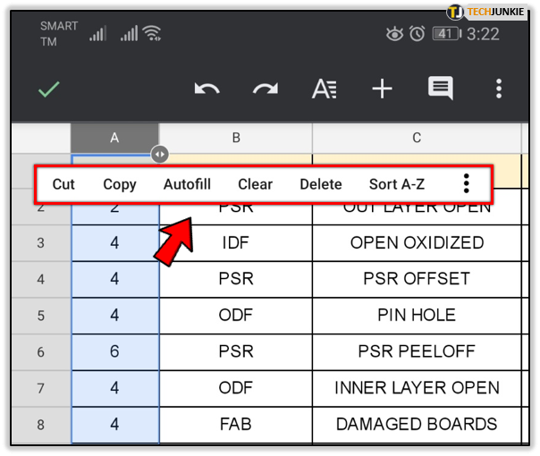
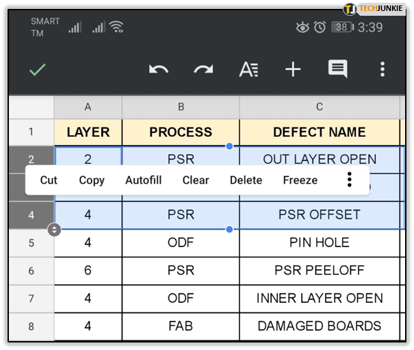
2. Long press on the selected row or column. When a menu pops up, choose either Freeze or Unfreeze to enable or disable sticky rows or columns.
   
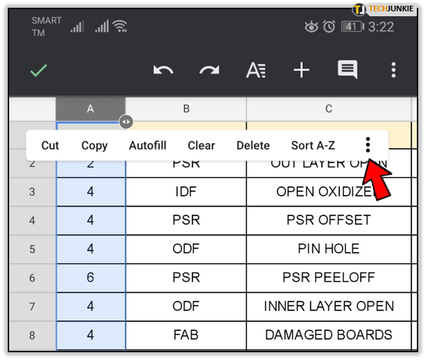
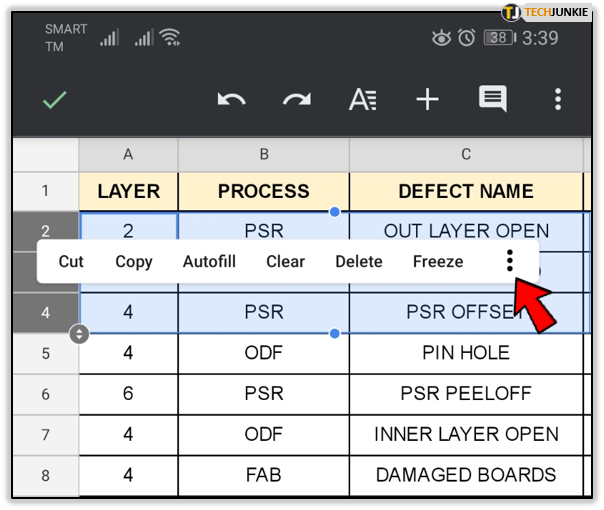
3. If you don’t see the Freeze or unfreeze command, tap on the three dots to the right of the menu to expand choices.
   

On iOS

1. Tap on a row or column letter to open the menu.
2. Tap the right arrow, then select Freeze or Unfreeze.

Hiding Rows or Columns

You can also choose to organize your spreadsheet by hiding rows or columns that you don’t want displayed. This will limit the number of rows or columns on view, and may be useful if you want to show the entire spreadsheet without having to resort to freezing.

To hide or reveal hidden rows or columns, do the following:

On PC

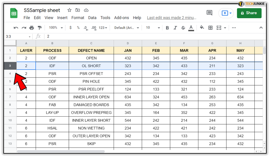
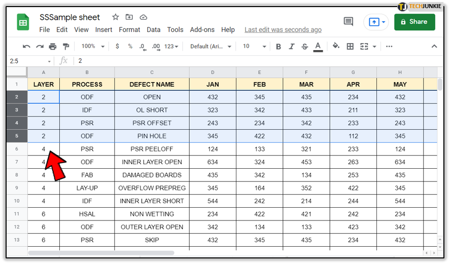
1. Click on a row or column that you wish to hide. If you want to unhide hidden columns or rows, click on the arrows on the row or column header to unhide. You can click and drag the mouse to select multiple rows or columns, or press and hold Ctrl while selecting them individually.
   
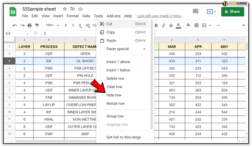
2. Right click on the selection, then select Hide Rows or Hide Columns as the case may be.
   
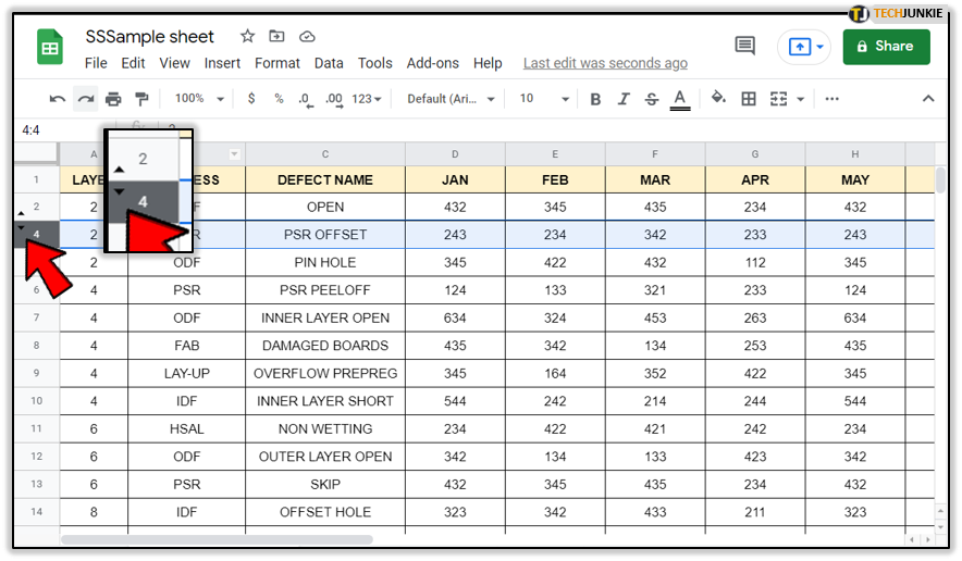
3. If your selection has hidden rows or columns, the option to unhide them will be available.
   
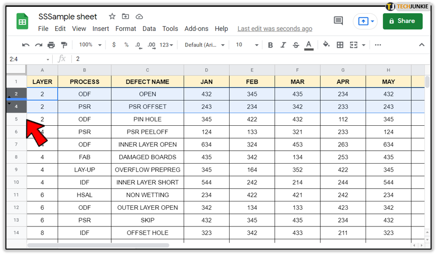
4. Hidden rows or columns will also be indicated by small up and down arrows in between the hidden data.
   

On Android

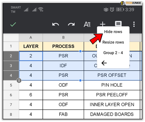
1. Long press on a selected row or column. To select multiple rows or columns, tap once, tap again and drag the blue lines, then long press to reveal the menu.
   
2. If you don’t see the Hide or Unhide command, tap on the three dots to the right of the menu to expand choices.
   
3. Tap on Hide or Unhide as the case may be.
   

On iOS

1. Tap on a row or column to open the menu.
2. Tap on the right arrow, then select and tap Hide or Unhide.

Grouping Rows or Columns Together

Another useful command to know is the Group rows or columns command. As the name suggests, this combines rows or columns into groups that you can then hide or unhide at will. This is quite handy as you can actually declare groups within groups, allowing you to make as many different group selections as necessary. To group rows or columns together, you can:

On PC

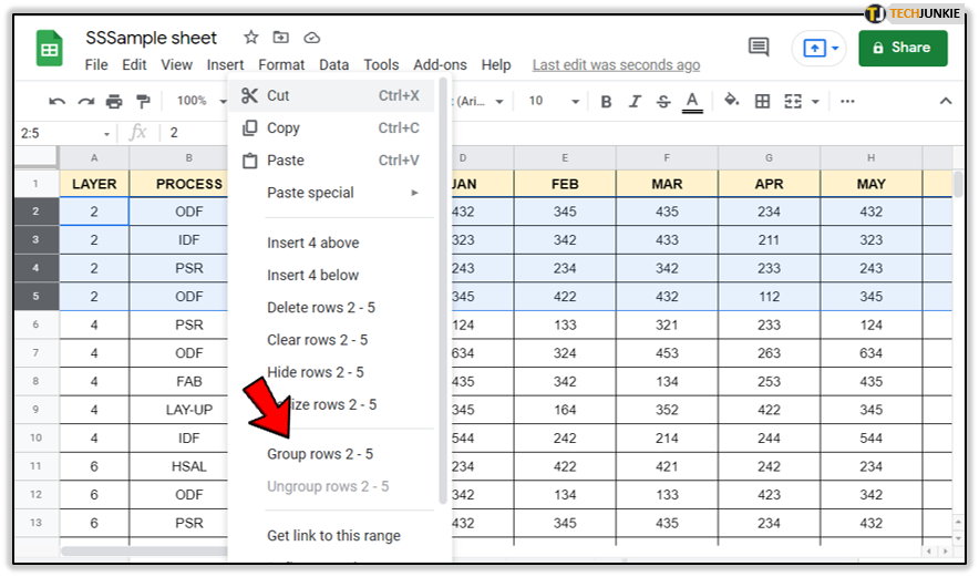
1. Select the rows or columns that you wish to combine.
   
2. You can either click on Data then select Group or Ungroup, or right click then choose Group or Ungroup to either combine or separate the rows or columns.
   
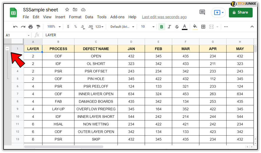
3. Pressing on the – or + symbols to the left of the sheet will either expand or collapse the groups selected.
   

On Android

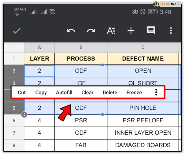
1. Select the rows or columns you want to group or ungroup, then long press to show the menu.
   
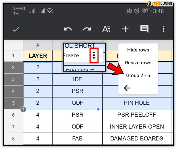
2. Tap on the three dots to expand the menu, then choose Group or Ungroup.
   
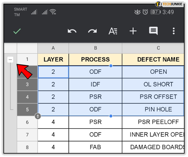
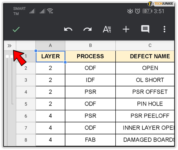
3. The + and – symbols to the left will expand and collapse the groups selected.
   
4. If there’s a group within a group, you’ll need to tap the double arrow symbol to expand it.
   

On iOS

1. Select the rows or columns that you want to group or ungroup.
2. Tap on the rows or columns, then tap on the right arrow on the menu that appears.
3. Select Group or Ungroup.
4. As with the other platforms, + and – will expand or collapse groups.
5. Groups within groups can be shown by tapping on the double arrows.

Useful Tools

Showing all the data of a worksheet may prove a challenge, especially for those that contain a lot of information. Being able to make rows or columns sticky, along with the hide and group commands, will surely make this process easier. These commands are useful tools for proper data management.

Do you know of other ways to make a row sticky on Google Sheets? Share your thoughts in the comments section below.