How to Unfreeze Columns in Google Sheets

If you’re working with a massive amount of data in Google Sheets, the option to freeze columns can be very useful. It’s a simple and effective way to prevent the data from a key column disappearing from your sight.

But if the sheet in front contains frozen columns that you’d like to unfreeze, there’s an easy way to do so. In this article, we’ll tell you everything you need to know.

How to Unfreeze Columns

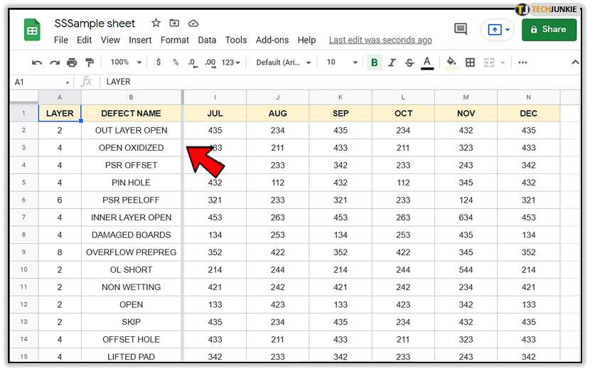
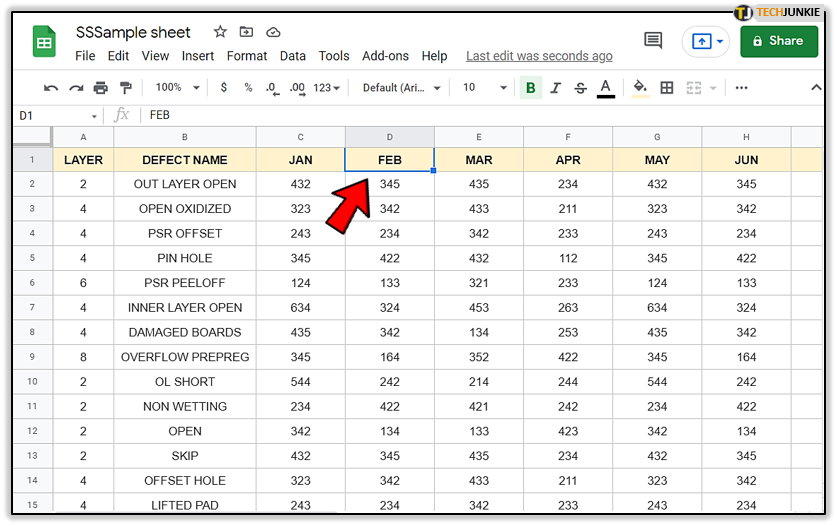
Here’s a simple sheet with numerous columns and rows. The first and second columns are frozen. If you scroll to the right, you can still see them.

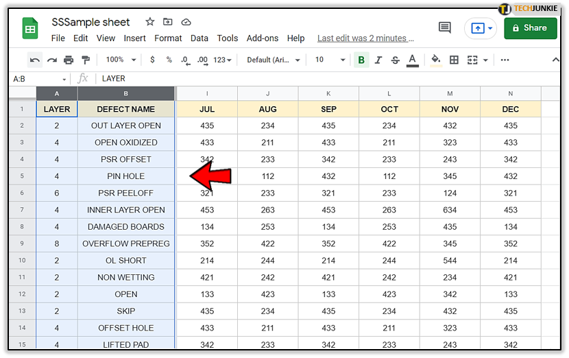
If you’d like to unfreeze this column, follow these steps:

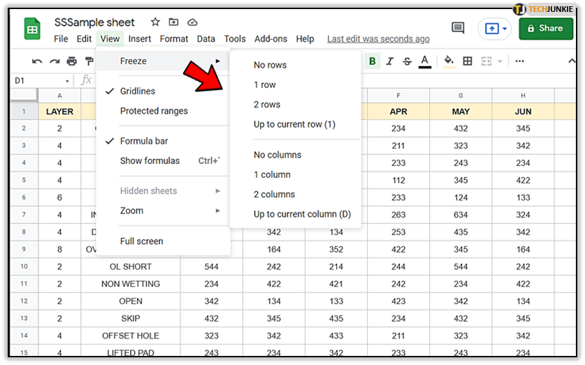
Press and hold Ctrl and select the columns you’d like to unfreeze (click if you’re working on a computer, touch and hold if you’re using Google Spreadsheets on Android, or tap it on your iPhone or iPad).
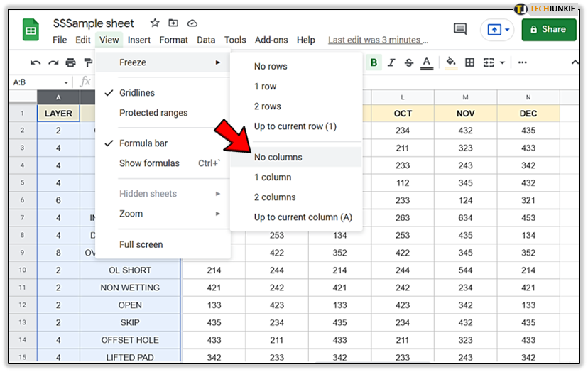
Click “View,” and on the drop-down menu choose “Freeze” > ”No columns”.

How to Freeze Columns

If you want to freeze those columns again – or to prioritize some other threads – the procedure is just as easy:

Select the column or click a cell on the column you want to freeze or keep visible.
Click “View”, choose “Freeze”, and decide on the number of columns that need to be frozen.

Note that you can also select either “Up to the current column” to freeze several columns at once.

Another Way to Freeze or Unfreeze Multiple Columns

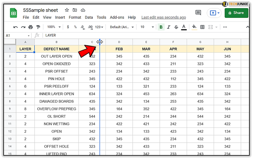
So you’ve frozen some columns, and now you’d like to freeze a few more. If they’re placed next to the already pinned ones, just drag the line that indicates the end of the last frozen column. Then, drop it where you want, to comprise other columns that need to be pinned.

It works the other way round too. You can unfreeze columns with drag and drop.

How to Customize Columns

When you create a new spreadsheet, all cells are the same. As soon as you start typing and entering data, based on the type of content within cells, you’ll probably need to change the width of columns, move them, insert new ones, or delete some columns.

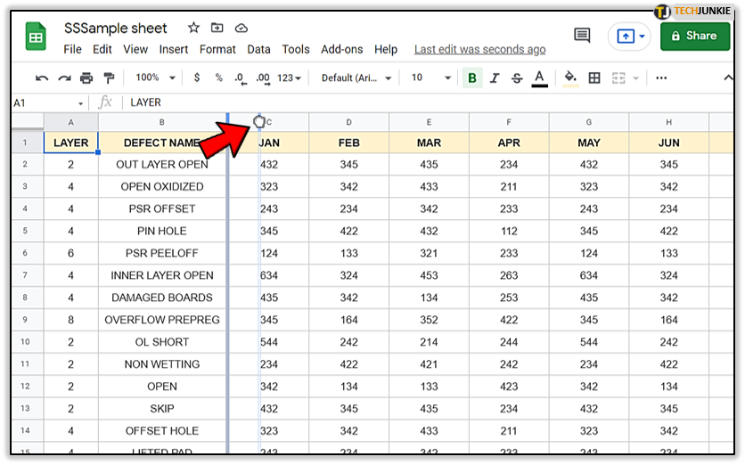
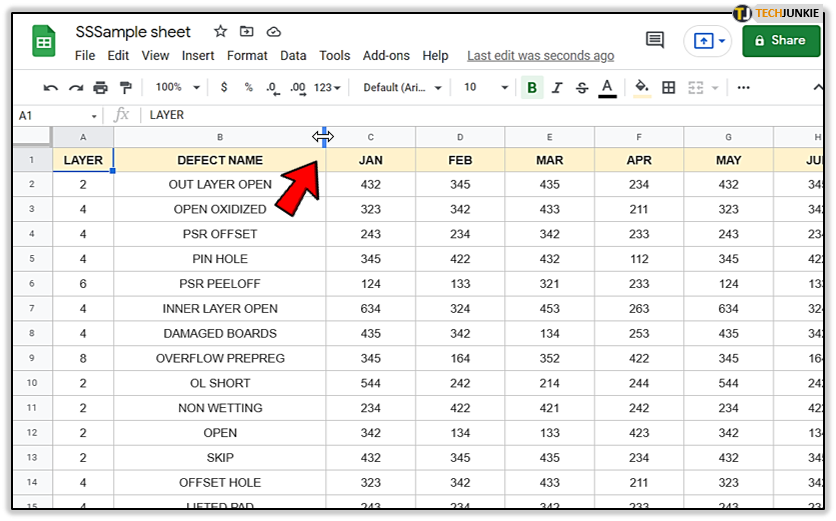
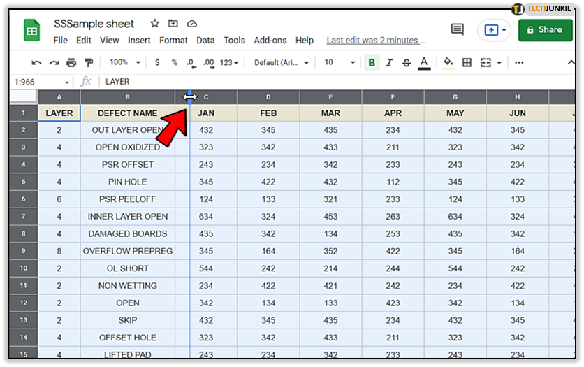
To change the width of a column:

Place the cursor on the right border of a column.
When a double arrow appears, click the border and move it to the right to expand, or to the left to reduce the width of the column.

If you’d like your column’s width to adapt the content, you can autosize its width. To do that:

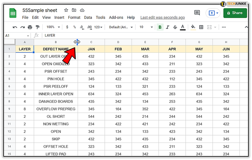
Place the cursor on the right border of a column.
When a double arrow appears, just double-click on it.

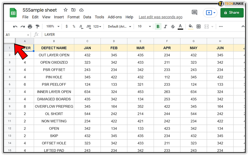
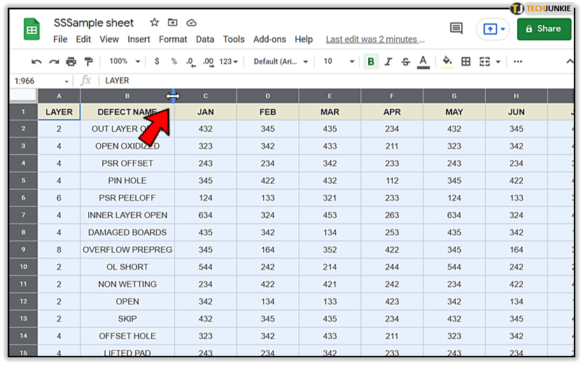
You might wish to make all your columns equal. To change the dimensions of all columns in a sheet at once:

Hold Ctrl and press A or click the blank button that’s placed just beneath the formula bar.
Place the cursor at the border of any column.
When a double arrow appears, click the border and move it to the right to expand, or to the left to reduce the width of the column – just like you would do with a single column.

Inserting Columns

To insert additional columns between the existing ones:

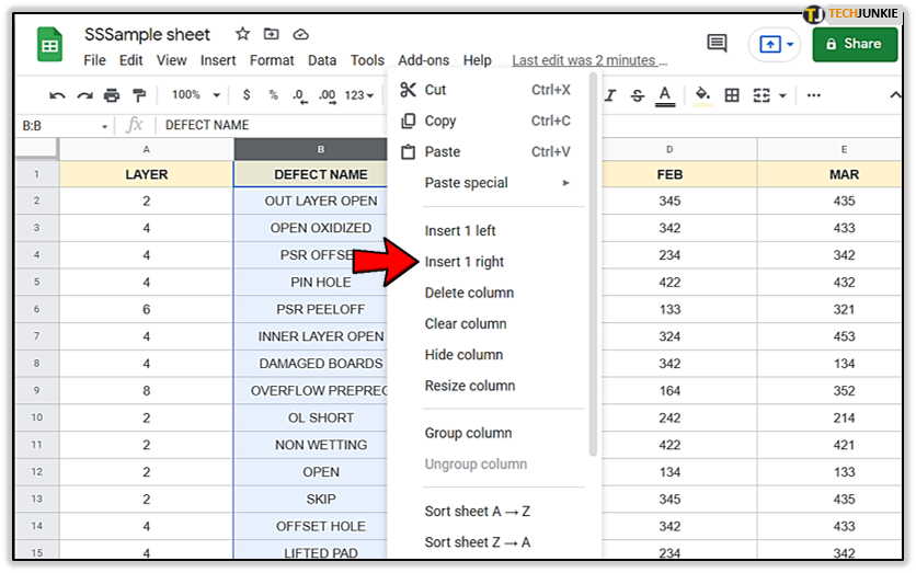
Select the column closest to the point where you want the new one to appear.
Right-click on it and then click either “Insert 1 left” or “Insert 1 right”.

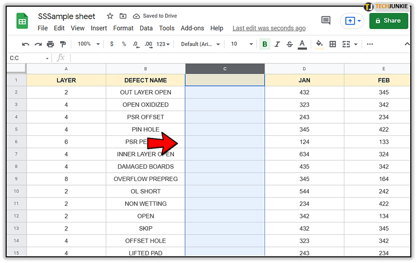
If you’ve reached the last column of the sheet, you can insert new ones as described above. But keep in mind that sheets have limits. The maximum number of cells in each sheet is two million. Even before you reach that limit, you might notice how everything slows down, especially if your sheet has plenty of complex models and formulas.

Pro Tip: Splitting Text to Columns

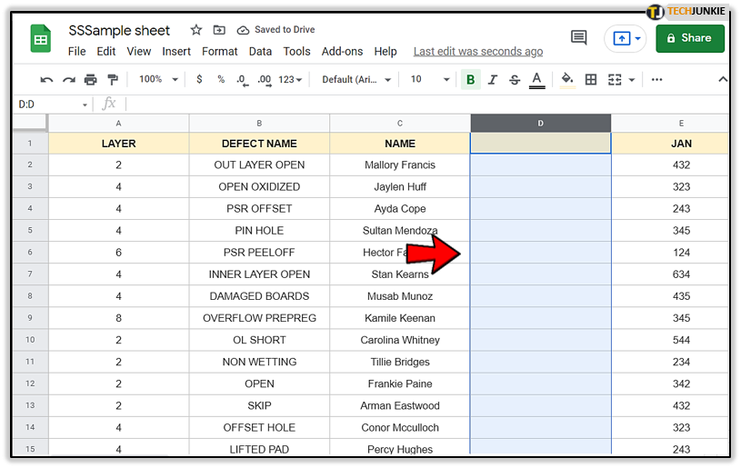
Imagine you have a column titled “Name” and you want to turn it into two separate columns – one containing first names only, and the other with last names. You could insert a column on the right and then move all surnames manually. But there is a better way to do this:

Insert a column to the right, as explained above.
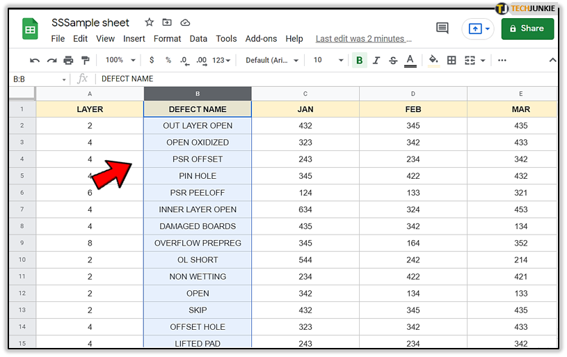
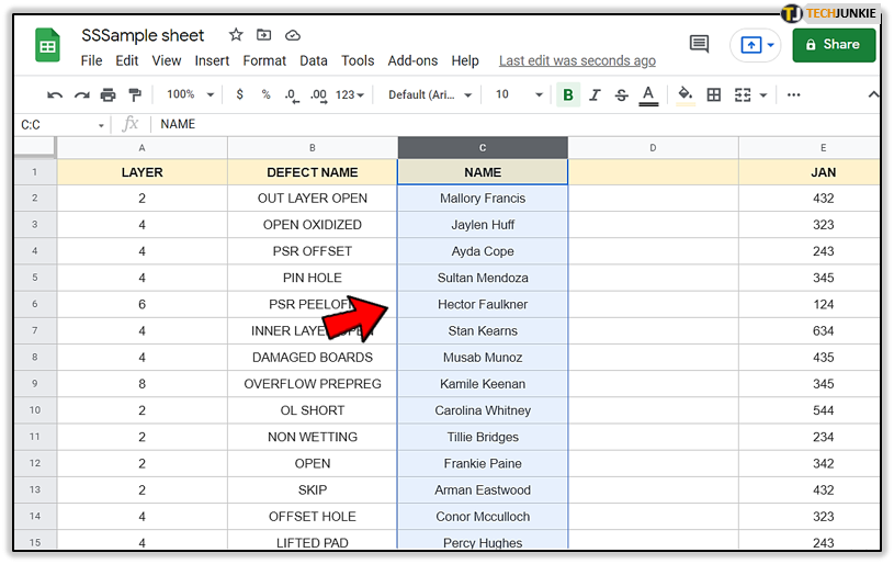
Select the column containing the full names.
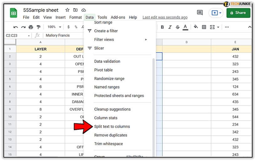
Click on the Data button and choose “Split text to columns” then select “Space” in the small pop-up box.
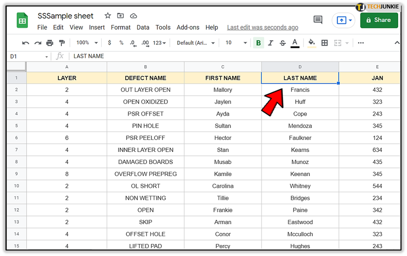
Rename the columns.

To Freeze or Not to Freeze

The option to freeze or unfreeze columns in Google Sheets can be really helpful if you’d like to keep the key data visible as you work. Unfreezing is easy – you can freeze and unfreeze as many columns as you like at any time. Whether you’re new to Google Sheets or a seasoned, advanced user, there will always be a column that you can freeze to make the whole sheet better organized.

Have you ever had to unfreeze columns in Google Sheets? Did you use the methods outlined in this article? Let us know in the comments section below.