

Google Sheets: How to Alternate Row or Column Colors

Something as simple as adding a checkbox in Google Sheets can make your spreadsheet a lot easier to work with. Google Sheets has many little-known features that will make you the king of productivity in your workspace. If you’re tasked with giving a spreadsheet alternating colors for a bit of flair, don’t even think about doing it manually as Google Sheets can do this automatically. With this guide, we’ll teach you how to alternate colors for rows or columns in a Google Sheets spreadsheet.
How to Alternate Row Colors in Google Sheets
Google Sheets has a unique feature that lets you automatically set alternating colors for rows and columns on a spreadsheet. First, learn how to do this for a row
- Open the spreadsheet in Google Sheets.
- Highlight the part of the spreadsheet you want to add colors to.
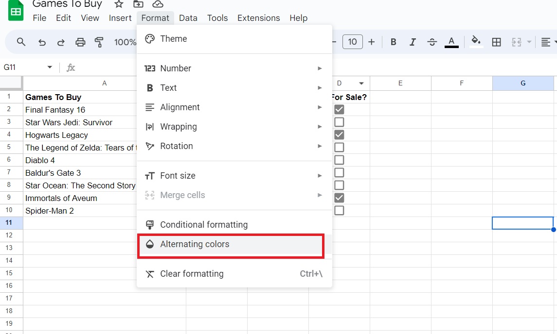
- Click Format and then select Alternating colors.

- Customize the colors as needed.
- Click Done once you’re finished.

You can integrate ChatGPT with Google Sheets to simplify your data analysis of the colored rows.
How to Set Custom Styles and Colors in Google Sheets
If you want to make setting up alternating colors in Google Sheets for rows or columns easier, use the Custom styles feature. With this, you can set up presets for colors that can be quickly applied to your cells in just a few clicks.
- Open the Google Sheets spreadsheet.
- Highlight the part of the spreadsheet you want to add colors to.
- Click Format and then select Alternating colors.
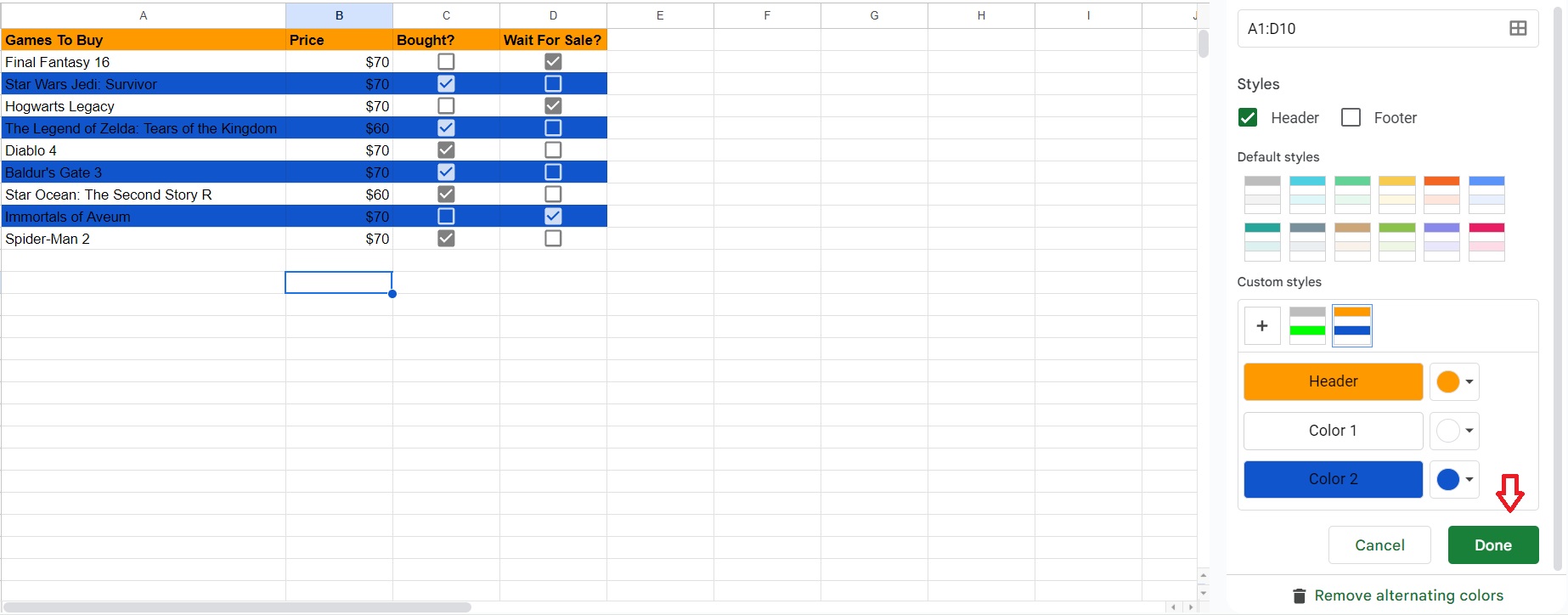
- Set the colors you want to use.
- Click the plus icon under Custom styles.

- Select the custom colors based on your preference.
- Click Done. The changes will be automatically applied after this.
You can split a cell in Google Sheets and then use custom styles to alternate the colors.
How to Set Alternate Colors to Columns in Google Sheets
Unfortunately, there’s no feature to set alternating colors for your columns in Google Sheets automatically. You need to do this manually.
- Open your spreadsheet in Google Sheets.
- Highlight the area to which you want to add the colors.
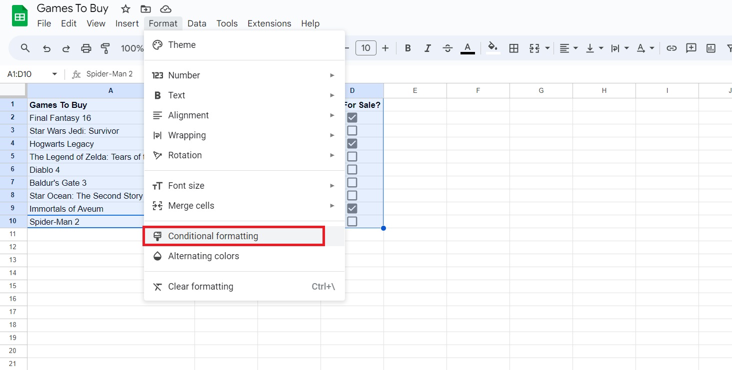
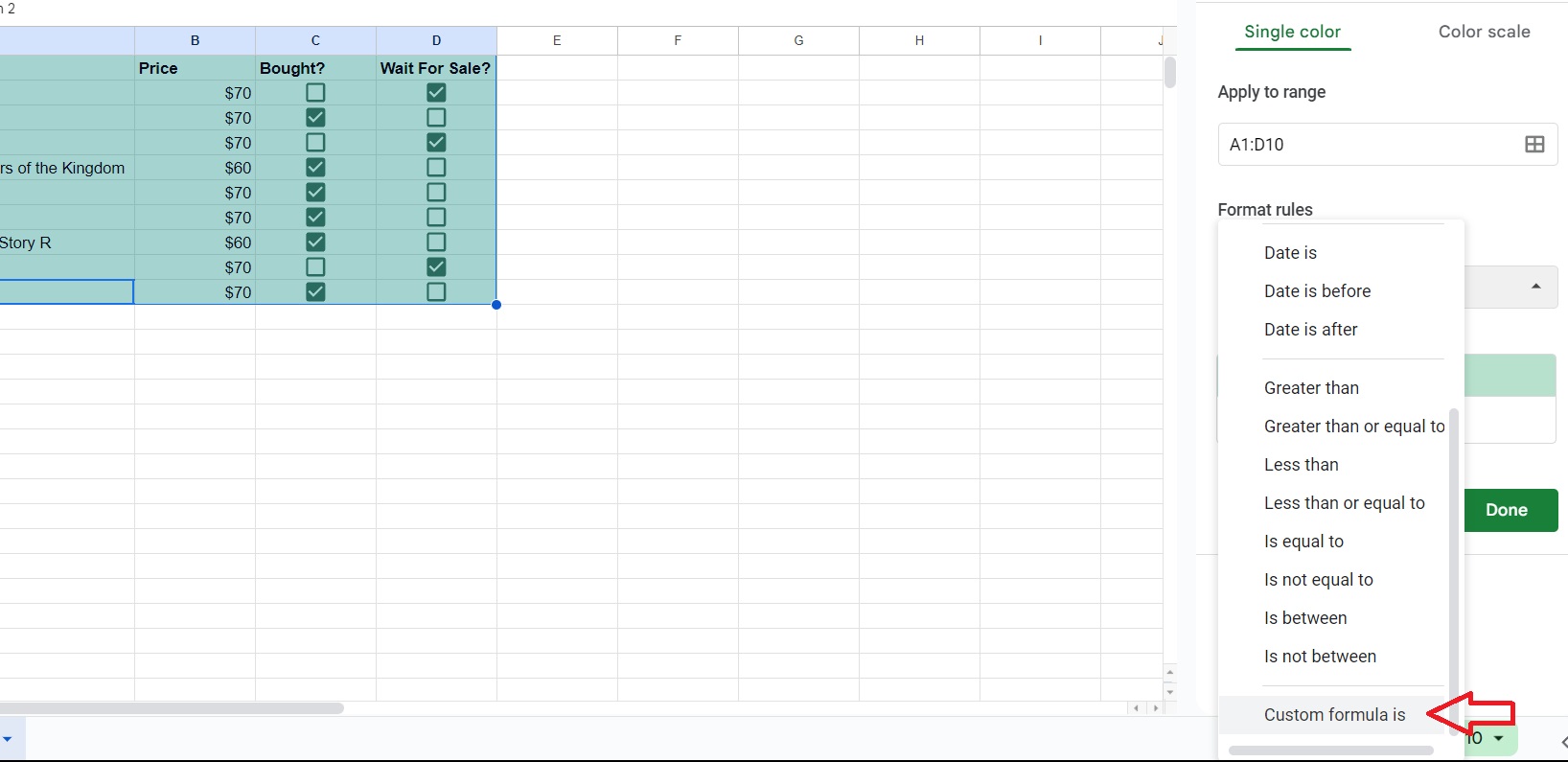
- Click Format and then select Conditional formatting.

- Click the drop-down menu under Format rules and click Custom formula is.

- If you want the colors to start in Column A, use this formula: “=ISODD(COLUMN())”. If you want it to start in Column B, use this: “=ISSEVEN(COLUMN())”.

- Click Done.
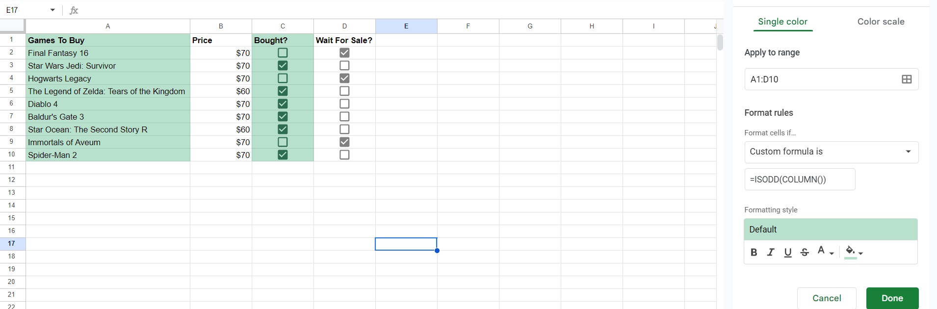
You can change the color by clicking the paint icon under Formatting Style.
How to Alternate Colors in Google Sheets on Android or iPhone
The good news is that you can also use the alternating colors feature from the Google Sheets app on your phone.
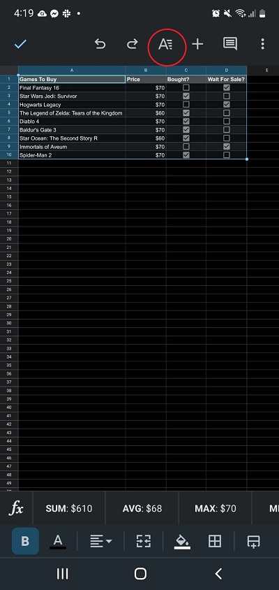
- Open the spreadsheet in the Google Sheets app.
- Highlight the cells to which you want to add colors.
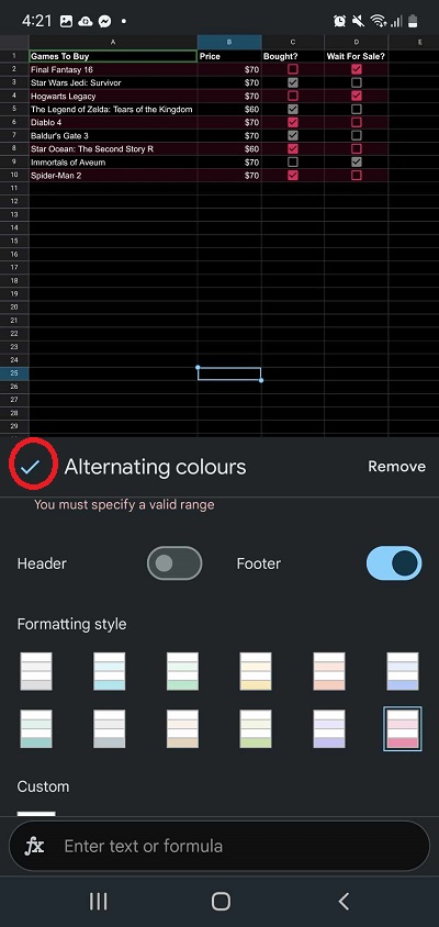
- Tap the Formatting icon at the top.

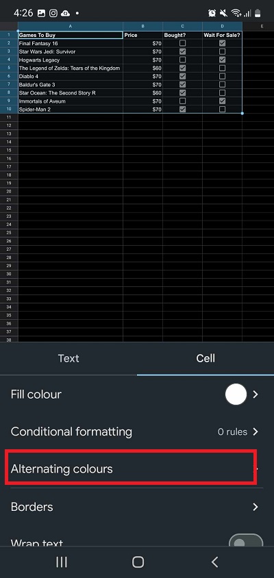
- Select Cell and then choose Alternating colours.
- Choose your formatting style.
- Tap the check icon to finish.
Give Your Spreadsheets More Life!
Adding colors to your spreadsheets doesn’t just make it look neater. You can also use this feature to organize your data on the file better. Presentation-wise, adding colors is going to make your spreadsheet less boring. For more Google Sheets tricks, here’s how to lock specific cells in Google Sheets so that others don’t accidentally mess with what you’re working on.
FAQs
A: The quickest way to do this would be to first highlight all the cells with colors you want to clear out. Once done, press Ctrl+/ on PC or Cmd+/ on Mac to clear formatting. This will also remove other formatting such as text colors, bold text, and more.
A: Yes, it is. You can access it from the Formatting icon located at the top. Select Cells, and then you should see conditional formatting from there. However, it’s more complicated, so we suggest using the desktop version of the sheets to access this feature.
A: Highlight the cell to which you want to add color. Click fill color from one of the options at the top menu. Pick any color you want; this should add colors to the cell you highlighted.