What Is the ISBLANK Function and How Do You Use It?

If you need to determine whether cells in Google Sheets are empty, you can do so manually. However, when you work with multiple cells, it soon becomes bothersome. Luckily, there’s a function you can use for this – ISBLANK. In this article, you’ll learn what exactly ISBLANK is and how to use this function. Let’s start!

What Exactly Is ISBLANK?

ISBLANK is a formula, which evaluates whether a cell in Google Sheets is empty or not. In a nutshell, it shows if there’s some value in the cell. But what are values? Well, these can be numbers, texts, or even another formula.

The ISBLANK formula shows if the cell is occupied by giving one of two answers: TRUE or FALSE. When there’s a value in the cell, the formula will show FALSE. For many, this can be confusing.

Shouldn’t it say ‘TRUE’ when there’s a value in it? That’s a good question, but think of it this way – you’re asking Google Sheets whether the cell is empty. When you get ‘TRUE,’ then it means it’s empty. But if you get ‘FALSE,’ then it means there’s some value in the cell.

How to Apply the ISBLANK Formula?

Learning any Google Sheets formula can be scary at first, especially if you don’t consider yourself a math or IT expert. But don’t worry, you don’t need to be super tech-savvy to use the ISBLANK formula. However, make sure to memorize the steps and don’t write any additional symbols to ensure the formula will work. Let’s see how to apply ISBLANK:

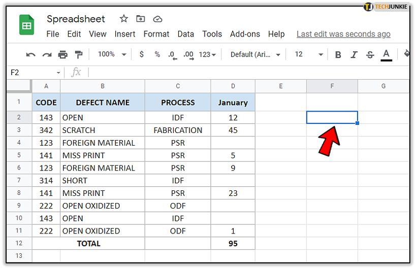
1. Open the spreadsheet you need.
   
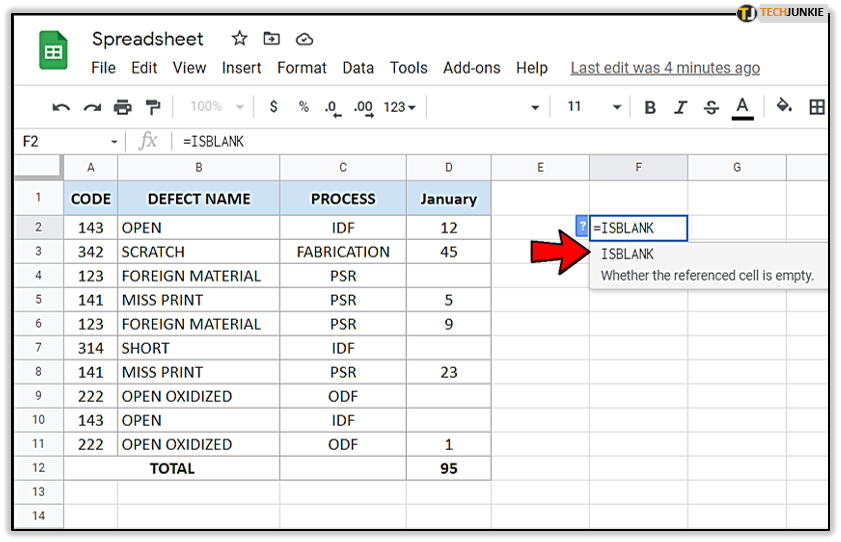
2. Click on a cell that doesn’t contain a value.
   
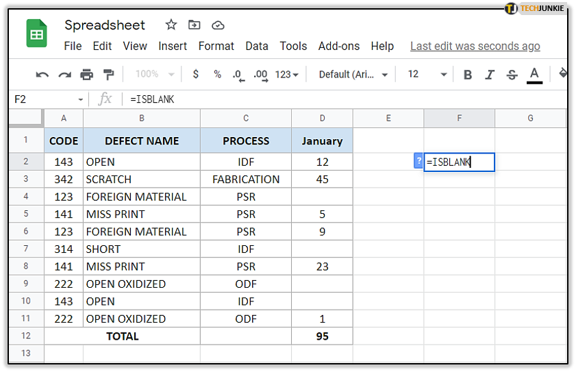
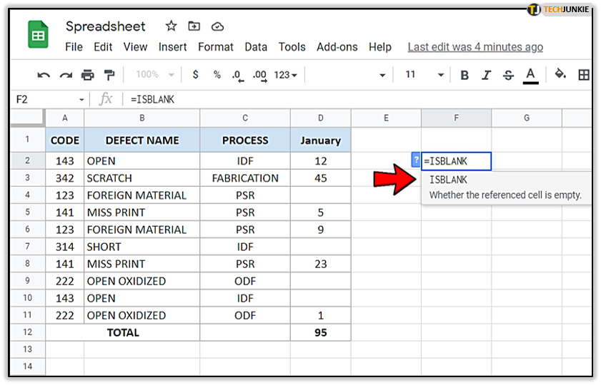
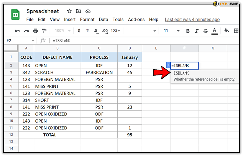
3. Now, in the cell you activated, type first ‘=’ and next to it ‘ISBLANK.’
   
4. You’ll see a box with ‘ISBLANK function. Click on it.
   
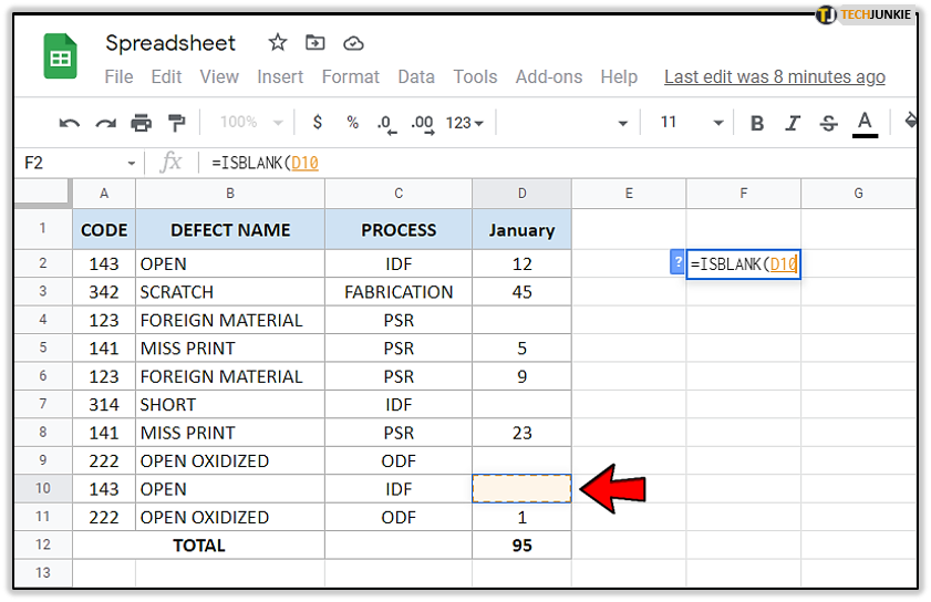
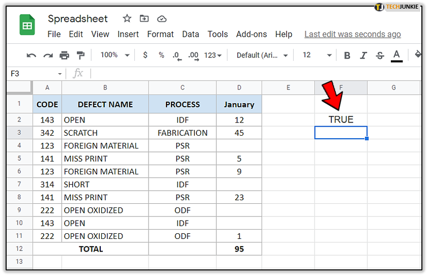
5. Now, click on the cell for which you want to perform this function. In this example, we clicked on D10.
   
6. Now, press ‘Enter.’
7. If you’ve followed the steps, then it should say ‘TRUE.’ This means that cell D10 is indeed empty.
   
   

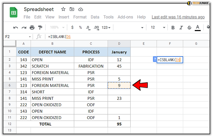
Let’s try performing the function for a cell containing some value:

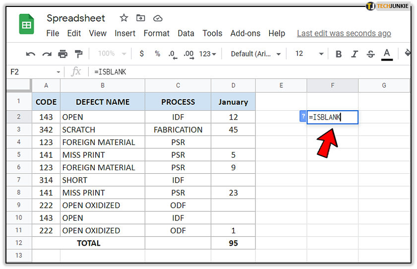
1. Once again, open the same spreadsheet.
2. Select the cell without any value.
   
3. Type first the equation sign ‘=’ and then ‘ISBLANK.’
   
4. You’ll again see a box with ‘ISBLANK function. Click on it.
   
5. Now, click on the cell with the value. In our example, we’ll click on D6 then hit enter.
   
6. Notice it says ‘FALSE.’ This means the cell isn’t blank.
   

There you go! Now you know how to check whether the cell is blank or not using the formula. However, some users have had issues with it. In the next section, we’ll explore them.

Issues with the ISBLANK Formula

“Why does the ISBLANK formula show ‘FALSE’ when there’s no value in the cell?” This is a prevalent problem Google Sheets users face. After following all the correct steps, somehow the formula shows the wrong result. In the main, it shows there’s some value, although the cell seems empty.

So, what’s the deal here? Is it a bug in the program? Most likely, that’s not the case. The reason is that you’ve accidentally entered whitespace. Or, you’ve hit ‘Enter’ and added a new line.

If you get an answer that doesn’t seem correct, go back to the cell causing problems and delete its content. Then, apply the formula again. It should show the correct answer this time.

Using the ISBLANK Formula to Check Multiple Cells

If you want to test a range of cells and see whether they’re blank, you don’t need to do this manually. The ISBLANK formula works for that, too. However, you need to combine it with the ARRAY formula.

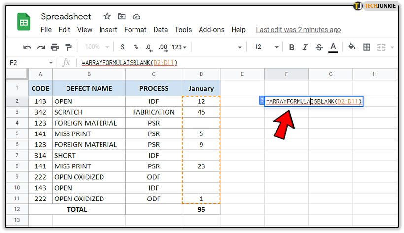
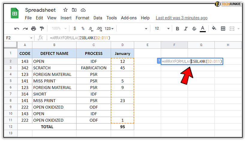
Assume you want to test a range of cells. Take a look at our example. We want to test cells D2:D11. This is how we’ll apply the formula:

1. Click on an empty cell to ‘activate’ it.
   
2. Then, type ‘=’ and ‘ISBLANK.’
   
3. You’ll see a box with ‘ISBLANK function. Click on it.
   
4. After that, use the mouse to drag down from the first cell to the last cell you want to test and insert a close bracket at the end of the cell range.
   
5. Now, type ‘ARRAYFORMULA’ after the equation sign.
   
6. Open a bracket after it, and make sure ‘ISBLANK’ is written inside.
   
7. Close the bracket after the bracket with cells and tap ‘Enter.’
   

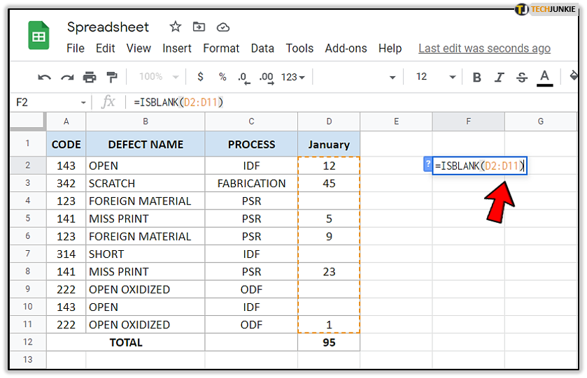
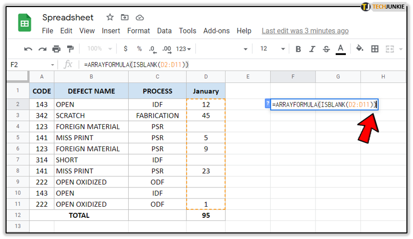
The formula should look like this:

‘=ARRAYFORMULA(ISBLANK(D2:D11)).’

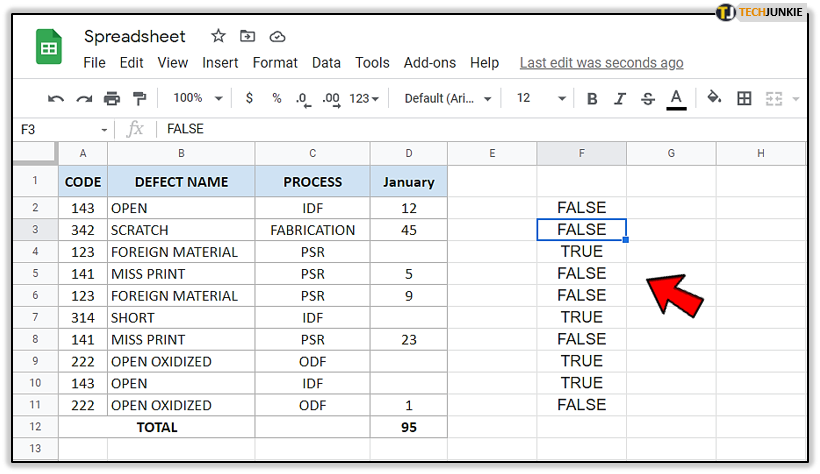
As you can see, with this function, you can check as many cells as you want. If you work with a lot of data, this kind of solution saves you a lot of time.

Learn the Formulas

Although formulas might seem tricky at first, they make life much easier. Memorizing the ISBLANK formula is a useful way to test multiple cells for values. However, make sure to remember that ‘FALSE’ means there’s a value in the cell you tested.

Which formulas do you usually use, and why? Have you ever had a chance to use the ARRAY formula? Share your experience with the community in the comments section below.